Thinking
About America’s Defense: An Analytical Memoir
Glenn
A. Kent
With
David
Ochmanek
Michael Spirtas
Bruce R. Pirnie
(c) 2008 RAND
|
Pages 12-13
In 1960, while working for General Gerhart, Glenn scored one of
his greatest coups. The Secretary of Defense at that time, Thomas
Gates, was interested in finding a means for imposing more cohesion
and integration on the nation’s operational plans for employing
nuclear weapons. Threatening the Soviet Union with a retaliatory
nuclear attack had for some time been the centerpiece of U.S. efforts
to deter a Soviet attack on the United States. Despite this, U.S.
plans for nuclear attacks on the Soviet Union and the Warsaw Pact
were not being developed in an integrated manner. Rather, they were
developed by the individual regional combatant commands and were not
well coordinated.
Charged by General Gerhart to involve himself in this problem,
Glenn played a pivotal role in conceiving of a process by which a
joint planning staff would develop an integrated plan. He called it
the SIOP. Working with Gen Thomas Power, who was then commander of
SAC, and Col George Brown, who was military assistant to Secretary
Gates, Glenn helped to choreograph the process for gaining the
secretary’s approval of this concept (see “The Advent of
the SIOP,” pp. 22–30). One result of the SIOP triumph was
that General Power, who had a reputation as fearsome as LeMay’s,
saw to it that Colonel Kent was eventually promoted to brigadier
general, in 1963.
[…]
In the summer of 1962, Glenn was assigned back to the Pentagon.
This time, he was working not for the Air Force but in the Office of
the Secretary of Defense (OSD). Specifically, he worked for Dr.
Harold Brown, who was then the Director for Defense Research and
Engineering (DDR&E). This was the heyday of Robert S. McNamara
and the “Whiz Kids”—analysts brought to OSD from
places like RAND. They were recruited in an effort to bring greater
rationality to defense decisionmaking through the application of
systems analysis. In Dr. Brown, Kent had a boss with a superb grasp
of mathematics and defense planning. Dr. Brown also enjoyed the trust
and confidence of Secretary McNamara. The Office of Systems Analysis
was headed by Charles Hitch and was home to many of the whiz kids. A
competition of sorts emerged between DDR&E and Systems Analysis.
Glenn had impressed Brown with some early work he did on issues
relating to the defense of the United States against nuclear attacks.
In time, Brown directed Kent—then a brigadier general—to
analyze the utility of the full range of programs for limiting damage
to the United States from a nuclear attack—offensive weapons
and delivery systems, active defenses (air and missile), warning
systems, and passive defenses (such as fallout shelters). This effort
consumed General Kent’s time for the better part of a year. The
study’s primary conclusion was that the U.S.–Soviet
strategic balance was dominated by offensive systems and that any
investment the United States might make in systems designed to limit
damage from a Soviet attack could be overwhelmed at less expense by a
larger attack. This insight led to a shift in policy that emphasized
ensuring a secure second-strike capability over limiting damage and
laid the conceptual foundation for two-sided arms control.
Pages 22 – 30
The Advent of the SIOP
In the 1950s, I
was a colonel heading the Weapons Plans Division on the Air Staff.
This division dealt solely with nuclear weapons and related issues.
It was subordinate to the Director of Plans, Maj Gen Glen Martin. He,
in turn, worked for the Deputy for Plans and Programs of the Air
Staff, at the time Lt Gen John Gerhart.
The United States
introduced nuclear weapons into its operational plans (OPLANs) in an
incremental and less-than-integrated manner. Different entities
developed their own OPLANs without much real coordination with
others. The Air Force developed a fleet of bombers capable of
carrying nuclear weapons. The Navy built submarines that could launch
intercontinental ballistic missiles (ICBMs) and also carrier-based
aircraft that were nuclear capable. Later, the Air Force created its
own array of ICBMs. The incremental nature of these developments
resulted in a less-than-integrated plan for how these weapons were to
be employed. The United States had no workable approach to unify the
planning among the various commands involved.
One
day, General Gerhart called me to his office. “There is an
ongoing item before the Joint Chiefs of Staff [JCS],” he
stated. “The Chief just told me that we cannot afford to lose
on this matter. I am hereby making you
the ‘action officer.’ Forget, for a while, about running
your division. Focus your entire efforts on winning this action
before the Joint Chiefs.” [*]
[* – For more detail on this debate, see Nathan
Twining, Chairman of the Joint Chiefs of Staff, memorandum to the
Secretary of Defense, “Target Coordination and Associated
Problems,” August 17, 1959.]
The
action before the JCS had been prompted by a memorandum from the
Chief of Staff of the Air Force to the JCS recommending that, to have
an integrated OPLAN for nuclear strikes on the Soviet Union, the
Strategic Air Command (SAC) should assume control of the Navy’s
Polaris submarines. The Navy and the Army were vigorously and
emotionally opposed to this recommendation. SAC was seen (rightly) as
an arm of the Air Force, and the Navy, in particular, had a tradition
of jealously guarding its autonomy. The fact that the Air Force, the
upstart among the services, had grown
rapidly under the Eisenhower administration intensified the
determination of the other services to prevent this expansion of
SAC’s authority. [*]
[* – In 1959, the Air Force’s share of the
DoD budget approached 50 percent. Since 1965, it has never exceeded
39 percent.]
The next day, I
discussed the matter further with General Gerhart. I told him that
the real issue was whether the United States should have one
integrated OPLAN or should just coordinate three plans: one developed
by SAC; one developed by the U.S. Navy Commander in Chief, Atlantic
Command; and one developed by the North Atlantic Treaty Organization
(NATO).
I then pointed
out that, to have a single integrated plan, it was not necessary to
place the Navy’s Polaris submarines under SAC or a unified
command. Instead, I recommended that the Air Force advocate the
formation of a joint strategic planning group. Personnel from all
services would staff this group. The commander of SAC would head the
group, and his deputy would be a Navy admiral. I also proposed that
this group be collocated with SAC in Omaha, Nebraska.
If
we want to prevail, I told General Gerhart, we must abandon the idea
of placing Polaris submarines under the control of SAC or even some
other specified command, a step that would provoke strong and
emotional opposition from the other services. Instead, we should
focus on the critical issue of a single
integrated operational plan (SIOP).
We could have a SIOP without grappling with the issue of command and
control over nuclear forces. General Gerhart agreed with this
approach and recommended to the Chief of Staff of the Air Force, Gen
Thomas White, and the commander of SAC, Gen Thomas
Power, that the Air Force change its position accordingly. They
agreed, though General Power was reluctant, and so the Air Force came
to advocate a SIOP and a Joint Strategic Targeting and Planning Staff
(JSTPS) in Omaha. [*]
[* – Thomas White, Air Force Chief of Staff,
memorandum to Secretary of Defense Thomas Gates, with attachment on
Strategic Targeting Authority, June 10, 1960.]
Both the other services opposed
our new proposal. In part, this was because the previous attempt to
gain operational control had poisoned the well. Even without this,
however, the other services would have been suspicious of the
proposal because they saw the SIOP and the joint planning staff in
Omaha as an ill-disguised gambit by the Air Force to dominate the
planning and conduct of nuclear operations, and they were determined
to prevent this. In their view, even our new proposal gave the Air
Force too prominent a role. They held that it was enough to
coordinate plans developed by the services. But we argued that the
United States needed a single plan, integrated from the beginning by
a joint planning staff.
The Secretary of
Defense, Thomas Gates, became aware of this issue and made it known
that he favored the approach being proposed by the Air Force. In the
interest of advancing the cause of integrated planning, Secretary
Gates asked his military assistant, Brig Gen George Brown (an Air
Force officer who later became the Chairman of the JCS), to keep him
informed of the status of this matter.
In an effort to
get the ball rolling in our direction, we proposed a trial run. An ad
hoc joint planning staff would convene in Omaha and develop a trial
SIOP to test the concept. The Navy opposed this proposal, but the
Secretary of Defense took affairs into his own hands and directed the
JCS to conduct this trial. After a month or two, the ad hoc planning
staff produced a first cut at a SIOP, but there was still
considerable dissension between the Air Force and the other two
services about a variety of issues.
There was a lot
to argue about. The Air Force wanted the plan to take into account
the possibility that poor weather would hamper or even prevent
operations by carrier-based aircraft. The Navy and the Army pointed
to problems regarding several issues having to do with Air Force
forces. They argued that far fewer bombers than estimated by SAC
would be likely to penetrate Soviet air space and reach their
targets. They also considered that the Air Force was far too
optimistic about the proportion of bombers that could be launched
before Soviet ICBMs destroyed them on their bases. In addition, they
argued that the Air Force was overestimating the hardness of Soviet
industrial targets. They feared that this assumption would have the
effect of raising the requirement for more nuclear forces and more
nuclear weapons.
In
an effort to force a resolution of these matters, the Air Force
submitted a memorandum to the JCS, proposing that the Joint Chiefs
and the Secretary of Defense convene in Omaha to review the draft
plan that the ad hoc planning staff positioned there had developed.
Predictably, the Navy and Army opposed this suggestion. Again, the
Secretary of Defense intervened. He directed that the meeting be
convened on December 18, 1960. In addition, he directed that the
objective of the meeting be changed from “review the plan”
to “approve
the
plan.” The Chief of Naval Operations was so strongly opposed to
this wording that he asked to see President Dwight Eisenhower. The
outcome of the meeting was predictable: The President sided with his
Secretary of Defense.
The ad hoc staff
had briefed the plan to the JCS in Washington several times in
preparation for the meeting in Omaha. The entire issue was nearing
some resolution, and it was certainly a top priority for all
concerned. The Air Force intended the following chain of events: The
draft plan would be briefed to all concerned (including Secretary
Gates) on December 18 in Omaha. The Air Force would then recommend
approval of the plan, with expected opposition from the Navy and the
Army. The Air Force confidently expected that the secretary would
decide in favor of approval, in light of the split, when the decision
was put to him. Thus, the plan would be approved.
But General
Gerhart wanted nothing left to chance. “How do we know the
Secretary of Defense will rule in our favor?” he asked. “We
must have a compelling argument to this end. You develop this
argument,” he told me.
Stuck
in traffic as I was going home that night, I pondered how we could
make an airtight case for our position. Then it struck me that the
right way to think about this was to view the SIOP as an OPLAN (which
it was) and as a means for making the best use of the forces
available—with not a hint as to any requirement to meet a set
of objectives. The plan should be presented as a set of allocations,
i.e., allocating this or that weapon to each designated ground zero
(DGZ). What effects
these
strikes would have and whether these were adequate to meet the
nation’s needs were important but separable questions. One
could argue endlessly about such issues as degradation caused by
adverse weather and darkness, the probability of our bombers
penetrating Soviet airspace, the hardness of the targets, what
portion of the Soviets’ industrial worth these strikes were
likely to destroy, whether these percentages represent enough
destruction or too much, and so forth. All these arguments tended to
be inconclusive because no one had the experience of all-out nuclear
war.
From the
perspective of a SIOP—narrowly defined—all these
arguments were beside the point. The task given to General Power and
his planners was straightforward: Make best use of the forces we
have. That meant that there was only one output: the allocation of
weapons to DGZs. The Air Force should declare that the sole purpose
of an OPLAN was to make optimal use of available forces, which our
plan did. There would inevitably be debate about the likely effects
of nuclear strikes and whether these strikes were adequate or not,
but these were separate issues.
Once this
position was staked out, the Air Force needed to show that the
protests by the Navy and the Army concerned the likely effects and
adequacy of nuclear strikes; they were not about the plan itself. To
this end, I proposed that General Power hold a meeting of the ad hoc
staff in Omaha. This meeting would include a two-star Navy admiral
and a two-star Army general. The participants in that meeting would
review all the items that were under protest by any of the services.
This would surely be a long and rancorous session. At the end of this
session, General Power was to inquire in a quiet manner whether the
Navy admiral or the Army general had any recommendations with regard
to the assignment of weapons to DGZs. If so, would they please submit
those recommendations to him?
We
hoped that the other services would make some recommendations, but
not too many. General Power would implement all their recommended
changes. At an appropriate time during the meeting on December 18,
General Power would state that he had asked for recommendations on
DGZs, that he had received certain recommendations from the Navy and
certain recommendations from the Army, and that he had changed the
plan to reflect all
these
recommendations. Therefore, he would declare that the plan itself was
not in contest. The likely effects of these nuclear strikes were a
topic for continued debate.
General Gerhart
liked this gambit. He told the Air Force Chief of Staff, General
White, about it and General White called General Power. Without
revealing any details over the phone, General White said that he
would send me to Omaha to explain the approach. I arrived at Offutt
Air Force Base (AFB) late that same evening and was promptly whisked
to General Power’s office. I explained to him the gambit that I
had proposed to General Gerhart. The central point was that the Air
Force be able to tell the Secretary of Defense on December 18 that
there was no protest about the plan itself.
“It
will work,” said General Power. “How many others know of
this gambit?”
“Only
General Gerhart and the Chief,” I replied.
“Then
keep it that way.”
We kept
everything under wraps until the meeting on December 18. On that day,
all the ranking civilians and military officers were in attendance at
SAC Headquarters in Omaha. In fact, General White, a four-star, just
made the cut to sit in the first row. The agenda items for the
meeting on December 18 all concerned various factors that could
change the predicted outcome of the nuclear strikes. As we predicted,
the participants engaged in a heated debate about these various
factors. Just before lunch, General Power requested the floor. He
stood in front of the group and spoke directly to the Secretary of
Defense. He explained the difference between factors that affect the
outcome of strikes and, on the other hand, the allocation of weapons
to DGZs. He said that, with respect to various factors, there was
much debate, but that with respect to the allocation of weapons to
the DGZs, there was none. He stated that he had accepted all the
changes proposed by the Navy admiral and the Army general about the
allocation of weapons to DGZs.
Secretary Gates
was more than impressed. He said, “General Power, if what you
say is true, then this casts quite a different light on this matter.”
He then extracted a grudging admission from the Navy admiral that he
had indeed submitted five changes concerning DGZs and that all had
been approved. He extracted a similar admission from the Army
general. The secretary then closed the discussion. He said that,
since there were no disagreements regarding the allocation of weapons
to DGZs, the plan should be approved without further debate, without
change, and today.
But the Chief of
Naval Operations, ADM Arleigh Burke, was not quite finished. “Mr.
Secretary,” he said, “I think that it would be rather
awkward if the Congress came to know that you coerced the Joint
Chiefs of Staff into approving the plan before it was officially
submitted to the Joint Chiefs for approval.”
Oh my. I had
overlooked this one important detail. The plan had been briefed to
the JCS three times, and the JCS had a copy of the plan. But the plan
had not been officially submitted to the JCS for approval. Any delay
would give the Navy time to recover. All the principals were
scheduled to depart the premises that afternoon and return to their
respective bases. Just as we seemed to have closure, it was slipping
away. There was no telling what would happen if the plan were not
approved during the session in Omaha. The Navy would recover and now
make some stern protest about the allocation to DGZs. I anticipated
that General Gerhart would not be pleased with this outcome or with
me.
Then Secretary
Gates came to the rescue. “Admiral Burke,” he said, “you
have a point to which I must react. The plan will be submitted to the
Joint Chiefs officially today. You will have all night to consider
it. I now amend my earlier statement. The Joint Chiefs will report to
me in the morning at nine o’clock as to which members approve
the plan and which members do not. If one member approves, I expect
the matter to be presented to me for adjudication. I will surely find
in favor of the member who has voted for approval.”
We were back on
track.
The Navy admirals
and Army generals protested about staying over in Omaha because they
had appointments to keep. The secretary brushed the objections aside.
“I expect to see each of you in this room tomorrow at nine,”
he announced. Then he asked, “General Power, may we partake of
your hospitality for one more night?”
General Power
beamed. “Of course. There will be a reception in the Officer’s
Club beginning at 1830 hours.”
At the reception
that night, General Power took me by the arm and ushered me into the
presence of General White. “General White, this is the man who
made this happen,” he said. From that time forward, I was a
protege of General Power, much to the benefit of my career in the Air
Force.
The
rest is history. In light of the secretary’s dramatic
statements, the Navy saw no value in continued opposition. At the
meeting on December 19, all three members of the JCS voted to approve
the plan. Once the decision was made that a JSTPS would be
established in Omaha for the purpose of developing a SIOP, the Navy
and Army worked hard to make the SIOP a
milestone in developing OPLANs. [*]
[* – Joint Secretariat, “Review of the
Initial NSTL and SIOP,” note to the Joint Chiefs of Staff on
JCS 2056/194, December 9, 1960. For more detail on the process of
creating the first SIOP, see Headquarters, Strategic Air Command,
“History and Research Division, History of the Joint Strategic
Planning Staff: Background and Preparation of SIOP-62,” n.d.]
This SIOP affair
was my crowning achievement as a colonel. It is a lesson that big
things can be accomplished by diligent and persistent staff
work—especially when the Secretary of Defense is on your side.
The following underlined my doctrine: Be sure your position in the
JCS is so compelling that, if there is a split, the Secretary of
Defense will surely rule in your favor. In this case, the key to
success was to conceive of a way to frame the debate such that
arguments against our position were simply untenable. It was clear
from the start that efforts by the Air Force to have the Navy’s
Polaris fleet “chopped” to the commander of SAC were
doomed. But the desired effect—greater coherence in the OPLAN
for executing the forces of both services—could be achieved in
a different, and more politically palatable, way. Who could argue
legitimately against a joint planning staff, especially when it was
made clear that the product of that staff—an OPLAN—was
intended to make best use of the forces available?
In later years,
SAC became simply Strategic Command (STRAT-COM), a joint combatant
command analogous to U.S. Central Command or U.S. Pacific Command.
And more often than not since then, the commander has been a Navy
admiral with submarines, bombers, and intercontinental missiles under
his control. This arrangement would have been unthinkable to all
concerned in the early 1960s. Time changes many things, sometimes for
the better.
In this episode,
the Air Force gained its point. The result was beneficial not only
for the Air Force but also for the country. Had the other services
prevailed, the United States would have gone on planning Armageddon
in a disjointed way. At best, planning by the individual services
would have caused inefficiencies, invited redundancies, and made the
nuclear deterrent less credible. At worst, such planning might have
caused uncertainty and ragged decision-making in a time of crisis.
Whatever parochial concerns may have motivated the Air Force to
advocate a single integrated plan, it was clearly in the national
interest. Finally, one might argue that the SIOP set a standard for
jointness that eventually expanded to conventional operations,
especially through the Goldwater-Nichols reform.
Pages 30 – 37
Defending the Planners of the SIOP
The time was the
mid- to late 1960s. Gen John McConnell was Chief of Staff of the Air
Force, and Dr. Harold Brown was Secretary of the Air Force. I was
head of Air Force Studies and Analysis (AFSA). General McConnell
called me to his office. He said that there was a big problem. Three
analysts from the Office of the Secretary of Defense (OSD) had made a
visit to SAC. They had been briefed on the SIOP and on the “planning
factors” used in the preparation of this document. They had
then written a report that was very critical of several of the
planning factors used by the JSTPS in developing the SIOP.
These analysts
had delivered their report to the Secretary of Defense, Robert
McNamara. The report included a recommendation that a group be formed
to thoroughly review how the JSTPS had developed the various planning
factors and how these planning factors were applied to defining the
SIOP.
General McConnell
went on: “This is not just an effort to improve the SIOP,”
he said. “These people have a hidden agenda. They have in mind
that the ‘review group’ they are proposing will declare
that the JSTPS at Omaha is inept and that this planning should be
done by a group reporting directly to the Secretary of Defense.”
The general added that he had been informed of the existence of this
hidden agenda by a very reliable source. He went on to point out that
events were moving rapidly. He and Dr. Brown had just returned from a
meeting with the Secretary of Defense. Secretary McNamara had
informed them that, in view of the report on his desk, he had little
choice but to form the group to review the planning. But General
McConnell saw this, and rightfully so, as a slippery slope. If the
group for the review were formed, there was a strong likelihood that
the responsibility for developing the SIOP would be taken away from
the JSTPS. He was determined that this whole affair be stopped in its
tracks.
General McConnell
went on about the discussion between Dr. Brown, the Secretary of
Defense, and himself. “While the secretary was explaining that
he had no choice,” he said, “it suddenly occurred to me
that I had a trump card to play. I recommended that the Secretary of
Defense not establish the review group until General Kent has had a
chance to review the critique by the people from OSD.”
The Secretary of
Defense accepted this recommendation. He knew me well from my days in
OSD under Dr. Brown. The general went on: “Your job is to show
that the analysts at Omaha are just as sharp as the analysts from
OSD. Show that there are serious flaws in the OSD report.”
At that point,
Dr. Brown entered the room. “I presume General McConnell has
told you of what happened,” he said. “I wish to
emphasize—there is to be no whitewash. Whatever your findings
may be, they must be able to stand up to critical review.”
Putting the two
statements together, my marching orders were clear: I must show that
SAC is right, that the OSD analysts are wrong, and the case must be
airtight.
A quick look at
the OSD report made it easy to believe General McConnell’s
statement about the hidden agenda. The critique was wide ranging. It
was obvious that the report’s authors were trying to establish
a basis for taking the responsibility for developing the plan away
from the JSTPS in Omaha. They had much more in mind than simply
trying to make some improvements to the SIOP itself.
As
noted in “The Advent of the SIOP” ( pp. 22-30), the SIOP,
in effect, defines the allocation of various nuclear weapons among
DGZs: Weapon number 22 goes to DGZ number 1; weapon number 23 goes to
DGZ number 2; and so on. In rare instances, more than one weapon is
assigned to the same DGZ. If you make a change in the SIOP, it is a
matter of changing weapon number 45 from DGZ number 21 to DGZ number
28. No big deal. The marginal return of making this change is
undoubtedly small and impossible to measure. The effect desired was
deterrence: That is, we sought to convince the Soviets that it would
be against their interests to launch an
attack. [*]
[* – Some people thought the effect desired was to
create unacceptable damage in a retaliatory attack. That may be so,
but it was always clear to me that we were better served by keeping
our focus on deterring a Soviet attack in the first place.]
In
this context, a change in the allocation of particular weapons would
result in little change in the degree to which we deterred—especially
if the Soviets were unaware of this change, which would be considered
Secret or Top Secret.
Now, back to the
OSD critique. The analysts identified, as I recall, ten issues that
they regarded as evidence of the JSTPS’s incompetence. One of
these (item 4) caught my eye: “The weight of effort allocated
to attack the Tallinn complex is ridiculous.” They actually
used these words verbatim. This intemperate language stood out and
made this item a likely candidate for rebuttal. If I could show that
the planners in Omaha were about right in this allocation, we would
have a leg up in tarnishing the report by the three OSD analysts.
The Defense
Intelligence Agency (DIA) had for some time—up to five
years—been reporting on worrisome activities by the Soviets
near Tallinn, the capitol of Estonia. Their estimate was that the
Soviets were installing an antiballistic missile (ABM) complex to
shoot down U.S. missile reentry vehicles (RVs) as they made their way
to targets in the Soviet Union. Activities had been observed at some
40 separate sites around Tallinn. DIA was not certain how many
interceptors had been deployed (or were to be deployed) at each site
and was not all certain of the effectiveness of each interceptor, but
it did give a range: between 20- and 80-percent effective—whatever
that meant.
The planners in
Omaha, in the presence of these tentative assessments by DIA, assumed
(1) that 15 interceptors had been (or might be) deployed at each of
the 40 suspected sites and (2) that each interceptor had around a
65-percent probability of kill (P_k) given a launch. In the presence
of these assumptions, the planners had allocated five RVs per site,
for a total of 200 weapons, to suppress the Soviet ABM system. It was
the number 200 that bothered the OSD analysts. It seemed like
overkill, especially in view of the uncertainty surrounding the
complex. Accordingly, they had labeled the allocation “ridiculous.”
In truth, at
first blush it does seem like overkill (allocating five weapons per
site)—if the lethality of each weapon is such that one is all
that is required to destroy all the interceptors at one site. But DIA
had stated that the probability of intercept might be as high as 80
percent (or words to that effect). The Soviets would use the
interceptors at the site in self-defense, and there would be only a
20-percent probability (at worst) of each U.S. RV penetrating, as
long as the ABM system is operating. So, it makes some sense to put a
sizable number of weapons onto the Tallinn ABM system to ensure that
the complex is destroyed and that the U.S. RVs attacking other DGZs
are not intercepted. The question remains: What is the optimum number
of RVs to commit to attack this complex?
I
began to consider ways to quantify the value of suppressing this
defense. Starting from the simple case of a single RV against a
single ABM site, we can calculate (on an expected-value basis) that
the RV would cause one interceptor to be launched in self-defense and
destroy 2.8 of the remaining Soviet interceptors:
0.2
* (15
- 1) = 2.8 (The
0.2 comes from 1 – 0.8.)
Thus,
11.2 Soviet interceptors would remain.
If
two RVs were allocated per site, 8.32 Soviet interceptors would
remain:
0.82
* (15
- 2) = 8.32
So
there is merit in allocating more than one RV per site. I saw that we
should expand these calculations to determine the “optimum
number of RVs per site.” My measure of optimum
in
this case was obvious: It is the number of RVs used in defense
suppression that maximizes the number of RVs that penetrate the
defense and proceed to attack other (non-ABM-related) targets on the
territory of the Union of Soviet Socialist Republics (USSR).
A
discussion with the planners in Omaha revealed that the weight of
effort (200 RVs) expended against the Tallinn complex had been
discussed—albeit very briefly—with the OSD analysts
during their trip to Omaha. The SAC planners were somewhat amazed
that the analysts had chosen the word ridiculous
to
characterize this allocation (200 RVs total). The SAC planners
pointed out that, if they assumed a probability of intercept of
around 65 percent, it took a little more than five weapons per site
to attain a damage expectancy (DE) of 0.90 per site. That is, 0.655
=
0.12, and 1 - 0.12 = 0.88 DE. And that was about the extent of the
discussion on that item.
During their
visit to SAC, the analysts from OSD did not challenge the number of
sites (40) or the possible number of interceptors per site (15),
mostly because the subject was not discussed in detail. Rather, they
challenged the requirement for 0.90 DE. They opined that while the
0.90 DE might have been sacred to the planners in Omaha, it had no
firm basis in policy or mathematical analysis.
I then undertook
a simple analysis. The measure of merit was the number of RVs to
penetrate the defense and reach DGZs in the USSR. Suppose that 1,000
RVs were involved in an attack. The planner would be willing to
divert 200 of these RVs to defense suppression if, by doing so, the
number of RVs available to attack other DGZs would increase.
The notional
characteristics of the Tallinn ABM complex were as follows:
1. 40 surface-to-air missile (SAM) sites
2. 15 interceptors per site
3. for a total of 600 interceptors.
Table 1.1 reveals
that, for the conditions stated, the optimum number of RVs per site
in defense suppression is between four and five. This allocation
maximizes the number of U.S. RVs that penetrate the Soviet defense,
as shown in the far right column of the table.
Table 1.1 Assessment of Allocation Options:
RVs to Suppress ABM Defenses
|
|
RVs
per Site (no.)
|
Defense
Suppression RVs (no.)
|
ABM
Interceptors – Not Fired (no.)
|
ABM
Interceptors – Surviving (%)
|
ABM
Interceptors – Remaining (no.)
|
U.S. RVs Destroyed (no.) [a]
|
RVs That Penetrate (no.) [b]
|
|
0
|
0
|
600
|
100
|
600
|
480
|
520
|
|
1
|
40
|
560
|
80
|
448
|
358
|
602
|
|
2
|
80
|
520
|
64
|
333
|
266
|
654
|
|
3
|
120
|
480
|
51
|
245
|
196
|
684
|
|
4
|
160
|
440
|
41
|
180
|
144
|
696
|
|
5
|
200
|
400
|
33
|
132
|
106
|
694
|
|
(a) – For a probability of intercept (PI) of 0.8.
(b) – The number of RVs launched less the number expended
in defense suppression less the number destroyed equals the number
of RVs that eventually penetrate the defenses.
|
So it turns out,
fortuitously, that the planning factor of 0.90 DE and a probability
of intercept of 0.65, as used by the SIOP planners, gave
approximately the right answer, though perhaps not for entirely
compelling reasons. But I was not obliged to defend the reason. The
OSD analysts in their report to the Secretary of Defense had not
directly challenged the use of a DE of 0.90. Rather, they had
challenged only the number of RVs diverted. So with regard to item 4,
OSD was wrong, and the planners in Omaha were right. I explained all
this to General McConnell and, in turn, to Dr. Brown. Dr. Brown went
through my calculations number by number and was satisfied that the
logic was sound.
Dr. Brown then
convened a meeting with the general, with the three OSD analysts who
had written the report and myself in attendance. I started with a
dissertation on the strategy to be followed when planning in the face
of uncertainty. I noted that planners must make choices about the
allocation of forces and that their choices must be predicated on
judgments about a wide range of factors whose precise values are
unknown. To be robust, a plan must be executable in the face of
adverse circumstances. Hence, the correct strategy is to maximize the
outcome for the case in which the factors in question are adverse. We
should, in the vernacular, “maximize the min.” We should
plan against the worst case. In this case, that meant planning for
the case in which the probability of intercept (PI) for the Soviet
ABM system was 80 percent. It would be imprudent to adopt a planning
factor that maximized the outcome when the PI was 20 percent.
Notice that I had
reduced the problem to whether the PI to use was 20 percent or 80
percent. This spread was derived from the DIA estimates. I announced
then that allocating five RVs per site, a total of 200 RVs against 40
sites, was about right for the factor of 0.80. I added that simple
math could be used to demonstrate this.
I had expected
that rather than challenge my math, the analysts from OSD would
challenge the assumptions about the structure of the complex I had
assumed—especially that the number of interceptors per site was
15. If one assumed that fewer than 15 interceptors were present, the
optimum number of RVs per site would be less than five. To my
surprise, they chose not to challenge either my math or my
assumptions. Instead, they declared that they were “not going
to get in a numbers game” with me.
I replied, “You
raised the issue of numbers. You stated that an allocation of 200 RVs
(five per site and 40 sites) was ‘ridiculous.’ My math
demonstrates that five is about right. Where is your analysis that
shows that five is so far wrong that it warrants the characterization
of ‘ridiculous’?”
At that point,
Dr. Brown observed that my confrontational tone was not conducive to
a productive discussion, whereupon General McConnell, to my surprise
and chagrin, stated that he agreed with the secretary and summarily
dismissed me from the room. As usual, the general was one step ahead.
In about 30 minutes, he called me to his office. “I got you out
of the room,” he said, “before they could change tactics
and try to challenge your analysis. After you left, I made the point
that, if they continued to pursue this matter, I would make the point
that they, when faced with your analysis, refused to be drawn into a
numbers game. I would certainly make this known to the Secretary of
Defense—and anyone else who would listen.” The general
went on: “While they did not agree to cease and desist, I think
we have heard the last of this matter. They, of all people, should
avoid making sweeping statements before they do their homework.”
And
so it was. Their report withered on the vine. They no longer pushed
the matter. Their choice of the word ridiculous
was
ill advised, and I had turned it into a fatal error.
In summary,
In
cases of this nature, it is almost always preferable to attack than
to defend. It would have been very difficult for me to show
convincingly that everything the JSTPS was doing was correct. At
best, this approach would have resulted in a series of charges and
countercharges with no conclusive resolution. But if I could
discredit the report of the OSD team, we might convince Dr. Brown
and Secretary McNamara to drop the affair.
If
you undertake to challenge or discredit a report, focus and dwell on
the one item about which its authors are obviously wrong and be
prepared to prove your point.
Never
use such polemical words as ridiculous
in
your own work unless the number you are challenging is very wrong
and you can prove it. Even under those circumstances, find a less
inflammatory word.
In the wake of
this episode, I was elevated to a higher stature in General
McConnell’s eyes. He would at times introduce me as his
“junkyard dog.”
Pages
37 – 42 – Calculating the “SIOP Degrade”
In 1991, Maj Gen
Robert Linhard was the Director of Plans and Resources at SAC in
Omaha. I had retired from the Air Force and was working at the RAND
Corporation. There had been some discussion in Washington about
deploying an active defense to counter any attack against the United
States by a third country (that is, one other than the Soviet Union)
with nuclear-armed ballistic missiles. Such a deployment would not be
consistent with the ABM treaty of 1972. Rather than withdraw from the
treaty, the United States was considering a concept that would allow
the Soviets to deploy a similar defense along their southern borders
to guard against an attack by their neighbors to the south.
General Linhard
wanted to know how such a defense, if allowed, would affect the
United States’ ability to execute the SIOP. In the terms he
used, he sought to understand the “SIOP degrade.” To this
end, he invited a group of analysts to convene in Omaha to address
this question. The invitees included analysts from the Los Alamos,
Livermore, and Sandia National Laboratories; two analysts from the
RAND Corporation (Dean Wilkening and myself); one representative from
the U.S. Arms Control and Disarmament Agency (ACDA); someone from the
Department of Defense (DoD) Office of Research and Engineering
(DDR&E); and others.
The meeting
opened promptly at 0830. General Linhard stated his question and
problem. The three analysts from the national labs set forth their
approach to answering the question. After further questions and
discussions, we finally disbanded for lunch. After lunch, General
Linhard opened with a statement: “What I learned this morning
is that, if I gave each of you a million dollars, after six months of
‘computer crunching,’ you could provide some tentative
answers.” They all nodded affirmatively.
At two o’clock
it was my turn. I opened by saying, “General Linhard, I am
prepared to provide you considerable insight as to the implications
of such a Soviet defense, this afternoon and for free. First, the
bottom line: The degrade to the SIOP will be minimal (something like
10 percent), provided (1) that you employ decoys based on the latest
decoy technology and (2) that you forbid the Soviets to deploy any
forward engagement radar in the northern part of their country (a
radar to control the engagement of a Soviet interceptor engaging U.S.
RVs).”
To scope the
problem,
1. Assume that each side is allowed no more than 200
interceptors.
2.
Assume that each interceptor has a P_k (for
a given engagement) of 0.7, for a total kill potential of 140.
3. Assume that the attack by Blue is 1,000 RVs against
1,000 targets, one RV per target.
4.
Assume that 1,000 targets contain people and industrial facilities
amounting to 1,000 units of “worth”—the proper
choice of a scaling factor can make this true. Note that, for
convenience, one unit of worth is an erdel (erdel
is
a fabricated word and means nothing).
5. Assume that the distribution of worth (erdels) among
the 1,000 targets obeys the distribution according to the equation by
the renowned economist Vilfredo Pareto, in which
V_cum = [ (n / N)^0.5 ]
* w
where
V_cum
is
the cumulative value, n
is
the stated number of targets, N
is
the total number of targets in the set, and w
is
the worth in the total set. The 1/2 is the exponent Pareto derived,
which of course indicates the square root. It follows that one-half
of the total value is in the first one-fourth of the targets.
Note that I was not breaking new ground with regard to
the distribution according to Pareto. Many analysts have used this
distribution, including the assignment of one-half as the value of
the exponent.
6. Assume that the Soviets are not allowed to deploy an
“engagement” radar to the north of the tier of provinces
in the south of their empire.
7. Without an engagement radar to the north, they cannot
engage in “threat-tube sorting.” That is, they cannot
determine the intended target DGZ of each attacking RV and thus
employ their 200 interceptors against the 200 RVs that are destined
for the 200 most lucrative targets. Note that the defense has great
leverage if it has a control system that provides this capability.
Without it, the defender has to engage the incoming RVs without
regard to the value of the target that each RV is intended to
destroy.
8. Also, by not allowing the Soviets to deploy an
engagement radar to the north, we assume that they cannot
discriminate between decoys and RVs in the attack by Blue.
For
the base case (no defense), the defense of course saves no worth
(zero erdels), and there is no degrade to the SIOP.
Now
take the case of a defense with a kill potential of 140 (200 *
0.7).
There are 1,000 RVs versus 1,000 targets, and each target contains
(on the average) one erdel of worth. Thus, the defense “saves”
140 *1.0, or 140 erdels. This amounts to a 14-percent degrade.
For the next
case, add 400 decoys to the attack. The decoys are, perhaps, Mylar
balloons and very light. Assume that we must allocate 20 weapon
spaces to employ the 400 decoys—a rate of 20 to one. The 980
remaining weapons attack 980 targets. These 980 targets contain 990
erdels:
1,000 * SQRT(980 /
1000) = 990
Now, with 400
decoys (and 1,380 total objects), the expected erdels saved per
object killed by the defense has been reduced from 1.0 to 0.717:
990 / 1,380 = 0.717
assuming
that the Soviet defense system is unable to distinguish between RVs
and decoys.
Then,
the erdels saved by killing 140 objects is equal to 100. To this
number, we must add the erdels saved by replacing 20 weapons with
decoys. This number is 10. So, the total erdels saved by the defense
is 110, and the degrade is 11 percent.
If
the technology of lightweight decoys permits 40 decoys per weapon
space allocated rather than 20, the degrade will be a little less.
The defense now “saves” less per object killed, 0.556
versus 0.717, as was the case for 400 decoys. Now, the defense saves
78 erdels (140 * 0.56)—plus the 10 erdels in the 20 targets not
attacked—for a total of 88 erdels, a degrade of slightly under
9 percent for the case of 800 decoys.
On the other
hand, if the Soviets can do threat-tube sorting, the problem takes on
a different complexion. With threat-tube sorting (and no credible
decoys), the Soviets would allocate their 200 interceptors to attack
(selectively) the 200 RVs that are directed toward the 200 most
lucrative targets. These 200 RVs put at risk nearly 45 percent of the
total value of the system of 1,000 targets. The expected value saved
by the defense per RV destroyed is now 2.25, and a kill potential of
140 saves 315 erdels. Now, the degrade is a whopping 32 percent.
We can see the
powerful reasons for outlawing forward engagement radars: (1) There
is no threat-tube sorting, and (2) there is no discrimination between
RVs and decoys.
At this point,
some of the other analysts could see their prospects for substantial
future work slipping away and proclaimed that the problem could not
reliably be reduced to such a simple calculus. Both General Linhard
and the gentleman from ACDA thought otherwise, and they stated that
they now had adequate insight to inform some key policy decisions:
1. Outlaw forward engagement radar (or radars).
2. Hold the number of interceptors the Soviets were
allowed to a low number—a few hundred.
3. Pursue a vigorous program to develop lightweight
decoys.
In the presence
of these three provisos, the problem of SIOP degrade was minimal and
presented no compelling argument against negotiating with the Soviets
to allow both countries to deploy a limited defense to counter the
threat of attack by third countries.
The key here is
to scope the problem and address the key assumptions in a manner
distinct from a focus on “computer crunching.” In other
words, just sit back and think. Often, doing this can provide a basis
for calculations that, while quite straightforward, yield new
insights into the most important aspects of the problem.
For reasons
external to those examined here, the whole concept of each side
deploying a limited defense was lost in the turmoil surrounding the
collapse of the Soviet Union and the United States’ decision,
in 2001, to withdraw from the ABM treaty of 1972.
Pages 43 – 50
Limiting Damage to the
United States
Early in 1964, a
study group was formed under the auspices of OSD’s Office of
Systems Analysis, headed by Dr. Alain Enthoven, to “look at”
a wide range of issues relating to U.S. nuclear forces and strategy.
Dr. Frank Trinkl was to run this group for Dr. Enthoven. At the time,
I was a brigadier general working in DDR&E for Dr. Harold Brown.
As someone with
experience in nuclear forces, I was asked to serve on this group. I
declined. In my view, there was next to no chance that this group
would succeed in providing insights useful for informing decisions on
the critical issues of the day. Several things were wrong:
1. There were far too many issues to address (18 in all).
2. There were far too many people involved. Some had been
called to the Pentagon on temporary duty and had no place to work.
3. There was no hint as to the analytical approach that
would be used to gain insight on any particular issue.
That I had
declined to serve was made known to Dr. Brown, my boss. He called me
into his office. I told him of my misgivings about the way the effort
was being run. He rather agreed but directed that I serve anyway and
do my best to make it a useful endeavor. To me, this amounted to a
mandate to try to reshape the effort.
My first
recommendation had to do with “grouping.” There were
several issues on the study group’s agenda that had something
to do with limiting the damage to the United States that might be
caused by nuclear attacks. Why not bundle them together under one
large effort called “limiting damage” and conduct a
comprehensive analysis of the prospects of significantly limiting the
damage to the United States from a Soviet attack and, additionally,
define the proper allocation of resources to the various means for
doing so? These means would include the following:
1. counterforce operations
2. active defense against ballistic missiles
3. active defense against bombers
4. passive measures (civil defense).
Dr. Trinkl opined
that such a study would require a major effort that he did not have
the time to undertake. I pointed out that I had not introduced any
new or additional items. I had merely laid out an analytical approach
to gain insight into a major and encompassing issue. Indeed, one of
the items he listed was just that: “limiting damage.”
Absent a comprehensive study, we were doing nothing more than
“looking at” several items without providing much-needed
insight on any one of them.
Dr. Trinkl
repeated that he was reluctant, given his time constraints, to
undertake the substantial effort I had proposed. He had ample reason
for this reluctance. Dr. Trinkl held fast, and so I departed the
group. I made sure that Dr. Brown heard of my decision (and of my
reasons for it) from me and not from someone else. He listened and
nodded. “You are right. Do the study yourself,” he said.
Ouch. I was now embarking on an effort that would consume most of my
time and energy for the next year or so.
The first thing I
did was recruit some good people. My choice from the Air Force was
Maj Jasper Welch. I knew him from earlier days. I asked a Navy
admiral I knew for the name of a Navy officer to serve on my team for
this huge effort. He mentioned a Captain Paolucci. “But you
don’t want him. He is something of a maverick. He is very smart
but can be difficult to work with.”
I thought for a
moment. “Send him down,” I said. “I would like to
talk to him.”
Capt Dominic
Paolucci opened the interview by interviewing me. “What am I
getting into?” he asked. “I don’t want to waste my
time working for another flag officer who doesn’t know squat
about analysis.” I explained my approach and showed him some
notional plots. Also, I added, we would try to provide insight as to
the allocation among the various means (players) based on marginal
return.
Captain Paolucci
was all ears and he began to get interested. “I would like to
serve,” he said. Recruiting Captain Paolucci was one of the
best moves I made. He was a brilliant analyst and became one of my
best friends.
After several
weeks, Major Welch, Captain Paolucci, and Captain Niemela of the
Army, using mostly notional data, produced a first cut, “proof
of principle” assessment of the primary options for limiting
damage from a Soviet nuclear attack. We presented this preliminary
briefing to Dr. Brown as an update about work in progress. To our
surprise, he then showed these charts to Secretary McNamara, who in
turn directed that there be a comprehensive effort with participation
by each service and, as well, the staff of the Civil Defense Office.
Suddenly, the
stature of the study went up dramatically. This was both good news
and bad news: The representative from each service was to be a
two-star general; I was only a one-star. There was also an effort to
establish a “steering group,” ostensibly to advise my
group on the conduct of the study. I deftly avoided such a group. We
were now engaged in a comprehensive study that was to have many
twists and turns.
One of the first
things to do was to get a better cut at the database for population
and manufacturing value added (MVA). A contractor laboriously went
through U.S. census data and defined circles in rank order as to
their “worth,” according to population and their value in
terms of MVA. The location of the first two circles was not
surprising: They were in Manhattan. Only one circle in California
made the first ten. At that time, California did not account for as
large a portion of the U.S. population or gross domestic product as
it does today. Moreover, even though the state ranked high in
population, it was quite dispersed. The circles, as I recall, had a
radius of five miles— approximately the lethal radius of a
1-megaton bomb.
So that was our
construct. The United States would strive to defend the worth in each
of these circles, and the Soviets would attempt to destroy it. We
assumed that the Soviets would attack where the worth destroyed per
missile expended would be greatest. These are the most lucrative
DGZs. Needless to say, this database became close-hold. The circles
were ordered in the first instance by population.
We also had to
consider the fatalities among the population from the radioactive
fallout from Soviet counterforce attacks on our nuclear forces, the
Minuteman silos in the Dakotas being the prime example. If the wind
came from the northwest, the debris from these attacks would cause
considerable fallout over Chicago and surrounding areas. To determine
the number of fatalities from this fallout, we had to make
assumptions about the proportion of the population that would seek
refuge in fallout shelters, the proportion that would survive if they
did, and the proportion that would survive without shelters.
We addressed the
Soviet bombers’ attack as follows: We would deploy enough
active air defense in sufficient numbers of interceptors so that the
Soviets would see no advantage in acquiring and deploying bombers as
part of their attacking force.
Obviously, there
were many assumptions to discuss (and argue) with the participants
from the services, each a two-star with a “dog in the fight.”
Finally, we had some answers. We were careful to state that the study
was not intended to predict the outcome of an attack with any
precision. Rather, it was intended to provide insight into two
issues:
1.
What are the prospects for limiting damage to the United States from
a determined and adaptive Soviet attack?
[*]
[* – We were careful to construct the analysis so
that the Soviet attack could be adjusted to whatever defensive
measures the United States put in place. Failing to do this would
have led to results that overstated the value of the defenses.]
2. What is the
proper (best) allocation of resources among the various “players”
involved in limiting damage:
a. civil defense with passive measures, such as fallout
shelters in many areas and blast shelters in the largest cities
b. active defenses against arriving Soviet ballistic
missiles with Nike-X
c. counterforce attacks with Minuteman missiles against
Soviet ICBM bases, submarine-launched ballistic missile (SLBM) ports,
and bomber bases
d. antisubmarine warfare operations with U.S. submarines
against Soviet SLBMs at sea
e. active defense with U.S. interceptors versus Soviet
bombers?
We
arrived at these allocations based on a marginal
return. [*]
[* – Unfortunately,
I have misplaced many of these graphs over the years, and they are
too complicated to reproduce now.]
We
finally published the study. The essence of the study is detailed in
Figure 2.1.
|
Figure
2.1 – Typical Allocations of U.S. Damage-Limiting Forces:
Soviet Second-Strike Countervalue
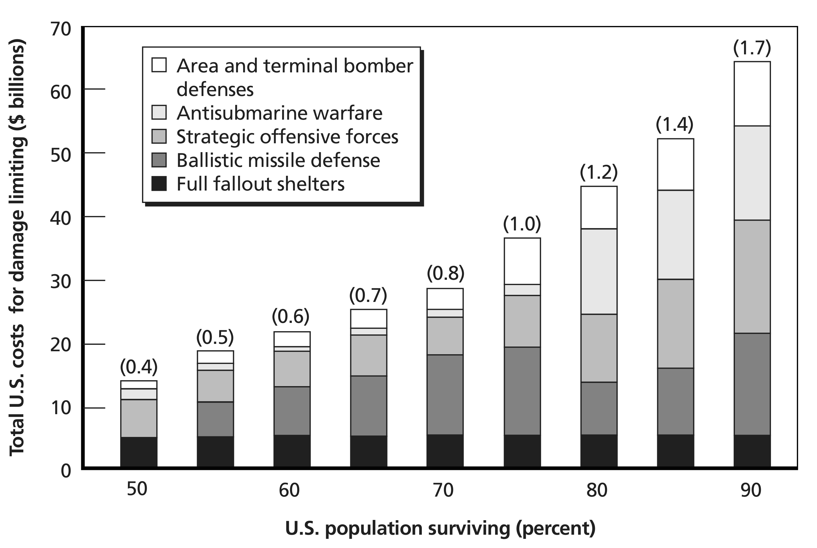
SOURCE:
Directorate of Defense Research and Engineering, A
Summary Study of Strategic Offensive and Defensive Forces of the
U.S. and USSR,
Washington, D.C., September 8, 1964, p. 120.
NOTES: For
each bar, the number in parentheses is the approximate ratio
between the cost of U.S. damage limiting and the cost of Soviet
damage creation.
In this
example, the Soviets allocated $12 billion for ICBMs, $16 billion
for SLBMs, and $9 billon for bombers, for a total of $37 billion
(FY 1965 cost estimates).
RAND OP223-2.1
|
The
figure shows, for each utility level,
1. the total
resources the United States must spend to achieve that utility level
in the presence of the stated Soviet attack
2. the
appropriate allocation of resources to each player
a. civil defense
b. ballistic missile defense (BMD)
c. strategic offensive forces
d. antisubmarine warfare
e. bomber defense
3. The ratio
between U.S. expenditures to limit damage and Soviet expenditures to
create damage as required to maintain the stated utility level.
For example, the
figure shows that, to achieve the level of 70-percent survival of the
U.S. population (against a stated Soviet deployment of ICBMs and
SLBMs), the United States would have to spend a total of $28 billion.
If the Soviets reacted to our deployments to limit damage by
deploying more ICBMs and SLBMs, the United States would be obliged to
spend more money to stay at the 70-percent level. The exchange ratio
(the amount the United States would have to spend to limit damage
compared to the amount the Soviets would have to spend to create
damage) was adverse to the United States. At the margin, it was
always cheaper to create damage than to limit damage. The graph shows
exchange ratios of 0.8 and 1.7, respectively, at the 70-percent and
90-percent survival levels. We realized (belatedly) that the
published numbers, which reflected the official exchange rate between
the ruble and the dollar, understated the exchange ratio. When the
values were revised on the basis that the costs to the Soviets to
purchase ICBMs and SLBMs were comparable to our own costs, the ratio
was more like 2:1 at the 70-percent survival level. At the 90-percent
level, the ratio was more adverse—probably 6:1. The charts
actually briefed to Secretary McNamara reflected the revised figures.
The secretary
observed that this was a race that we probably would not win and
should avoid. He noted that it would be difficult indeed to stay the
course with a strategy that aimed to limit damage. The detractors
would proclaim that, with 70 percent surviving, there would be
upwards of 60 million dead.
The secretary
went on: Instead of seeking unilaterally to limit damage, we should
undertake to negotiate a treaty with the Soviet Union to curtail the
deployment of nationwide defenses. This could set the stage for
agreements to control the deployment of offensive forces. Needless to
say, this was a statement of great and lasting strategic importance.
So my efforts to
gain insight into options for limiting damage had an unexpected
ending. Rather than reordering priorities for investments among
approaches to limiting damage, the study resulted in a rather
fundamental change in policy that led the administration to more or
less abandon efforts to limit damage in a meaningful way.
“Limiting
damage” did not appear as a stated strategic objective in the
draft presidential memorandum (DPM) issued in 1964.
Pages 50 – 54
Limiting Damage:
Allocation of Resources
As stated
earlier, the study on limiting damage addressed the question of the
proper allocation of resources among the various “players”:
1. Civil defense
2. BMD
3. strategic offensive forces to engage in counterforce
operations against Soviet ICBMs in silos and Soviet SLBMs in port
4. antisubmarine warfare forces to conduct counterforce
operations against Soviet submarines at sea
5. air defense forces (both area and terminal defenses)
to intercept Soviet bombers.
The allocations,
in general, were based on marginal return. All the players operate
with diminishing returns, and we have the optimum allocation when all
players are operating with the same marginal return, that is, when a
stated increment of funds yields the same increase in the measure of
merit (U.S. population surviving) regardless of the player to which
this increment is granted.
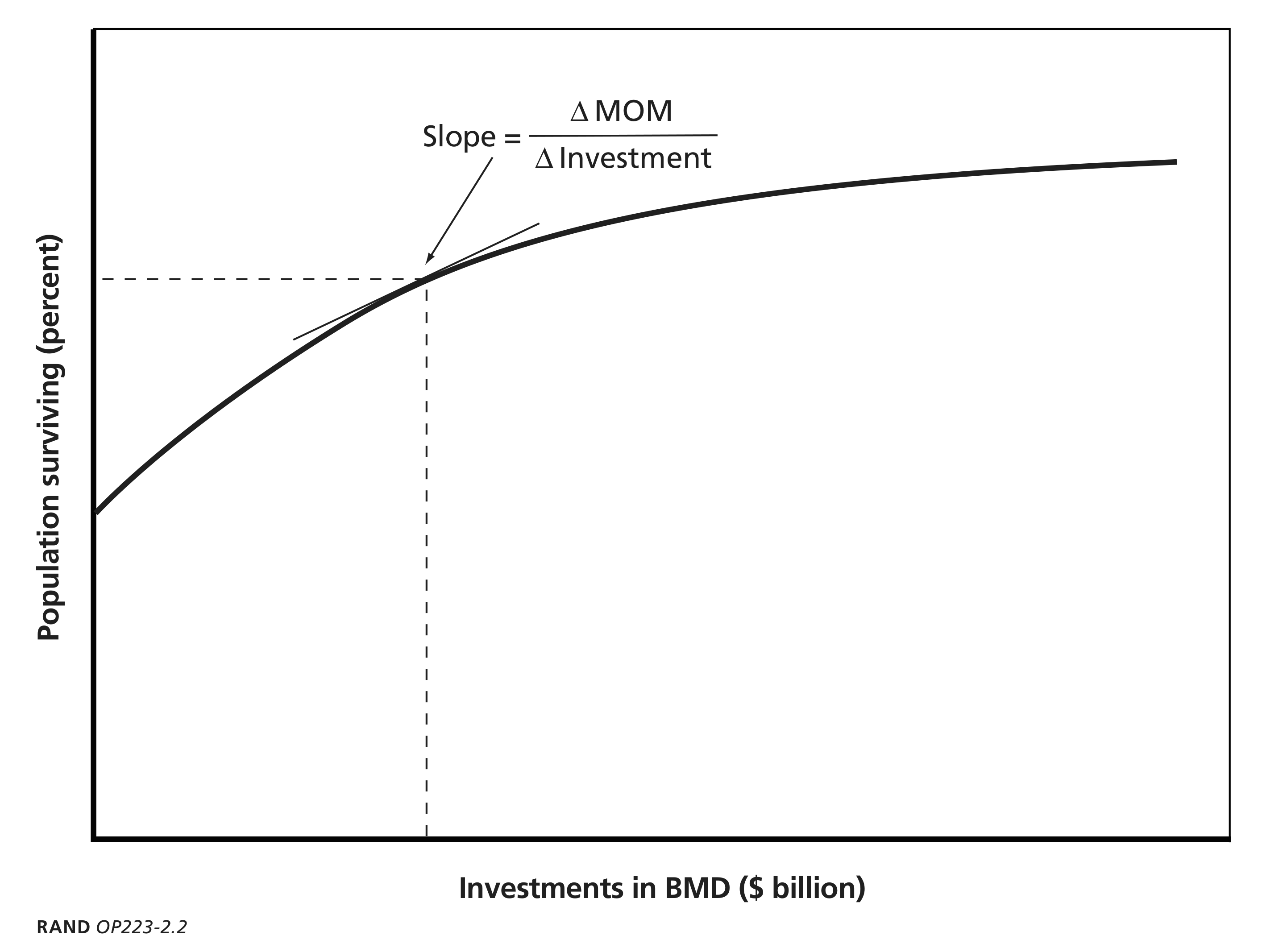
We determined the
optimum allocations using graphs. We plotted graphs with the measure
of merit on the ordinate and money allocated to a particular player
on the abscissa. Once the graph was plotted, we could take a ruler
and determine the slope of the line at any particular level of
expenditures allocated to that particular player. The slope, by
definition, is the ratio of the change in the measure of merit to the
change in investment, where the measure of merit was either the
population surviving or the MVA surviving (see Figure 2.2).
|
Figure
2.2 Relationship Between Investments in BMD and U.S. Population
Surviving (notional)
RAND OP223-2.2
|
We created such a
plot for each of the five players. It was, to say the least, a
complex, iterative, and laborious approach. But the team persevered,
and finally, we arrived at a point at which, with reasonable
confidence, we could state the optimum allocation of resources among
the various players.
For example, we
concluded that, for the stated size of attack, the United States had
to spend a total of $28 billion for 70 percent of the population to
survive. That $28 billion should be allocated as follows:
$5.2
billion to civil defense
$12.8
billion to active BMD
approximately
$6 billion to strategic offensive forces
approximately
$1 billion to antisubmarine warfare
approximately
$3 billion for bomber defense.
Today, with
high-speed computers, the optimum allocation to each player (at
various levels of total expenditures) could be determined more
quickly but not necessarily more reasonably. We conducted many
excursions to test the proposition that allocations other than the
ones we stated as optimum would yield worse results in terms of the
measure of merit (U.S. population surviving).
One challenge of
note regarding allocations stemmed from a group of people on contract
at the Civil Defense Agency. They were charged with evaluating the
concept of constructing blast shelters in the largest cities. We
chose not to implement this concept even though, at the higher level
of expenditures on BMD, the marginal return was equal to or better
than the slope for BMD for population surviving. What disqualified
blast shelters from our final comparisons was that, unlike every
other player, they offered no protection to the economic
infrastructure of the United States. In short, when the measure of
merit is MVA surviving, blast shelters for the people were not
considered a player. Since BMD operates on both of the measures of
merit, the nod goes to BMD. Not surprisingly, the Civil Defense
Agency contractors were not convinced and continued to challenge our
decision not to recommend that this concept be implemented. As it
turned out, none of the concepts were implemented. In this sense, one
could say that the operation (the analysis) was a success, but the
patient (limiting damage) died.
Another challenge
regarding allocations came from the representative that the Air Force
assigned to my study group. We had stated that, in each of our
optimum allocations, the United States should provide the capability
to employ one effective RV against each Soviet ICBM silo. This was an
increase from the planning factor of zero set forth in the DPM,
developed by Dr. Enthoven. This was not a new issue. Dr. Enthoven
argued, with some traction, that the United States, as a matter of
policy, would not engage in a first strike. Thus, in any conflict,
most of the Soviet ICBMs would already have been launched before our
RVs arrived. This meant that our counterforce attacks against these
empty silos would have minimal effect in reducing the number of
Soviet ICBMs arriving at U.S. targets.
Our analysis on
limiting damage revealed that counterforce operations with Minuteman
RVs (one Minuteman per Soviet silo) were a viable option, even if
only 20 percent of those silos still housed an ICBM when the
Minuteman missiles arrived. We stated that we could not predict with
any certainty how a future exchange might unfold.
Still, in the
presence of this uncertainty, we should adopt a planning factor of
one RV per silo.
Dr.
Brown and Dr. Enthoven were impressed by this argument, and it was
agreed that DoD would revise the planning factor up from zero to one.
But the Air Force representative, a two-star general, wanted more. He
argued for a planning factor of two RVs per Soviet silo. To bolster
his position, he argued that the Pk
of
a Minuteman RV against a Soviet silo was 0.9. We had used 0.6 for the
Pk, and with good reason.
I
pointed out to the Air Force general that the marginal return of the
second Minuteman RV would be minimal, as the Pk of the first RV was
0.9. This was so because 0.9 times 0.1 (the residual value of the
silo that had already received an RV) is 0.09. If you choose to argue
for two, I said, then you should allege that the Pk
is
0.5, since x
times
1 - x
is
at a maximum when x
=
0.5. Still, the general held to the position that, if we would just
use 0.9, the stage would be set for a planning factor of two, when in
fact alleging that the Pk
was
0.9 destroyed any argument for the second weapon. As a matter of
fact, a Pk
of
0.6 was not far off from 0.5 in terms of the marginal return of the
second weapon: It was 0.25 for a Pk of 0.5 and 0.24 for a Pk
of
0.6. Nevertheless, the Air Force general refused to grasp the
disconnect in his train of logic.
He had other
complaints as well. He bundled them together and proclaimed to the
Chief of Staff of the Air Force (then Gen Curtis LeMay) that I was
“selling the Air Force down the river.”
General LeMay
convened a meeting, the stated purpose of which was to determine
whether or not I was selling the Air Force down the river. General
LeMay began the meeting by stating his intention to demote me back to
colonel. At that meeting, the two-star presented his case—including
the issue that he had submitted that the Pk was 0.9 and I
had ignored his input and used 0.6. In my response, I dwelt on this
point. Fortunately, General LeMay saw the disconnect in the logic
presented by the two-star, namely that a Pk of 0.9 did not
set the stage for a planning factor of two. In fact, it was the other
way around. I pointed out that I had convinced Dr. Brown and Dr.
Enthoven of the merit of allocating one Minuteman RV to each Soviet
ICBM silo—up from zero. I pointed out that the issue of using
0.6 for the Pk as a planning factor was hardly any
evidence that I was selling the Air Force down the river. As a matter
of fact, it was quite the contrary. At this point, General LeMay
abruptly ended the discussion and departed the room. The crisis
abated, and I heard no further word on this matter.
Pages 54-56
Helping with DPMs
During the tenure
of Secretary Robert McNamara, there was, as I mentioned above, a
document known as the “draft presidential memorandum.”
Actually, it was none of these things. It was not a draft; it did not
go to the President; and it was not a memorandum. Nevertheless, it
was a defining document whose focus was on defense strategy and the
associated means. It defined objectives and the strategy we would use
to achieve them. It also discussed the means and capabilities we
intended to use to implement our strategy and the forces we intended
to field to gain these operational capabilities—all in
considerable detail. It also contained programming data, such as the
amount of money allocated to each program element in the budget to
field these forces.
All the above was
administered by the Planning, Programming, and Budgeting System
(PPBS), then run by Dr. Charles Hitch, formerly of RAND. Dr.
Enthoven, also formerly of RAND and who reported to Dr. Hitch, was
responsible for writing the portion of the DPM that dealt with
strategic nuclear forces and strategy. The overall construct was a
marvel of clear thinking. The section by Dr. Enthoven was invariably
logical, insightful, correct, and short—on the order of 30
pages. I was heavily involved in the preparation of the strategic
nuclear section simply because of Dr. Brown. Dr. Hitch had to gain
approval from Dr. Brown, and Dr. Brown consulted me on what was to be
stated in this section.
I
address the matter of the DPM not to chronicle my part (which was
secondary) but rather to compare this document and to contrast its
development with the approach used today. Documents in the mid-1990s,
such as the Report
on the Bottom-Up Review and
the Secretary of Defense’s annual reports, compare favorably.
But not so today; the Strategic Planning Guidance recently issued is
300 pages long, and it fails, in my judgment, to define in clear
terms either our strategy or the means we intend to use to implement
that strategy.
Dr. Hitch, Dr.
Brown, and the secretary himself would review the DPM, item by item
and line by line. In addition, the Chairman of the JCS and the
service chiefs conducted their own review. Their comments were taken
seriously, but they held no power of veto.
One example in
particular illustrates the clarity of the document. The document
stated the administration’s paramount strategic objectives: to
deter strategic nuclear attack by the Soviets on the United States;
to limit damage from such an attack if one should take place; to
deter the Soviets from launching an all-out attack on Western Europe;
and, if necessary, to halt such an invasion as far forward as
possible (i.e., near the intra-German border).
Our strategy with
respect to the first objective, deterring the Soviets, was to have
the operational capability to inflict severe damage on the USSR. We
gained this capability by deploying SLBMs on submarines at sea, by
deploying weapons on bombers on quick alert at bases in the United
States, and by deploying nuclear weapons on ICBMs in hardened silos
in the United States.
Prior to the
completion of the damage-limiting study, our strategy with respect to
limiting damage was to increase our operational capability to conduct
counterforce operations against Soviet ICBMs in silos and SLBMs on
submarines in ports, to deploy an active defense against incoming
Soviet RVs and bombers, and to construct a stated number of fallout
shelters (but no blast shelters). From this point, having laid out
the basic defense strategy, the DPM dealt mostly with programming
data.
The
DPM was indeed a defining document in shaping the direction the
United States was to take—both with respect to strategy and
with respect to means. The DPM reflected the decisions of the time
and was revised annually until it was eliminated by Secretary Melvin
Laird during the Nixon administration. The DPM of 1963 included some
definitive guidance as to measures the United States would take to
limit damage. In the DPM of 1964, these statements were quietly
absent, a change stemming from the study on damage-limiting
I had conducted. [*] In light of that study, Secretary McNamara had
decided against allocating large amounts of resources to the various
means of achieving that objective.
[* – For more detail, see “Limiting Damage to
the United States,” pp. 53—50.]
Over the years, I
had, from time to time, several arguments with Dr. Enthoven, some of
which were quite heated. On the other hand, I always applauded his
skill and insight in drafting the DPMs. We would do well to emulate
his approach and construct today.
Pages 137 – 139
The Short-Range Attack
Missile Affair
Another program
that incurred unneeded turmoil as a result of the misuse of the term
requirement was the program to develop a shortrange attack missile
(SRAM) for the B-52 strategic bomber. The program began in the
mid-1960s. The concept was to equip the B-52 with a nuclear-armed
missile to attack a Soviet SA-3 air-defense site with impunity. The
SRAM would be fired at the site from a distance beyond that at which
the SA-3’s radar at the site could detect and track the B-52.
The calculation
for the “required” range was straightforward. At 23 nmi,
an aircraft flying at 400 feet above ground level cannot be detected
and tracked by a radar on a 90-foot tower with a grazing angle of 6
degrees to the horizon. At a lesser range, the radar could detect and
track the aircraft. So the 23 nmi range was indeed an operational
requirement. If the range of the missile was less than 23 nmi, the
SA-3 battery could not be attacked with impunity, and the concept
would be null and void.
A development
program was commenced. By about the late 1960s, the SRAM was
approaching initial operational capability (IOC). I was in AFSA at
the time. A colonel from another office brought in a report for my
coordination. It was an annual report to Congress as to the status of
the acquisition programs the Air Force was conducting, system by
system. For each system, there was an item called “Requirement.”
To my surprise, the “requirement” listed in this document
for the SRAM was that the missile have a maximum range of 37 nmi. I
had been involved in framing the concept for the SRAM some years
before and remembered that calculations determined the maximum range
to be 23 nmi. After some investigation, we learned that the switch to
37 nmi came from a calculation by an engineer at Boeing, the prime
contractor for the program, who determined that the system they were
building would have “thrust” and “drag” such
that it should be expected to fly 37 nmi. I pointed out that this
longer-range figure was a statement about expected performance, and,
harkening back to my earlier experiences, I added that there was some
danger in putting it down as an “operational requirement.”
The colonel agreed in good faith to change the draft he was
coordinating to state that the requirement was 23 nmi, but his
superior, a general running the directorate for “requirements,”
overruled him. “Why put down 23 nmi when we are on contract for
37?” he reasoned. They did not inform me of this decision.
A year went by. A
new annual report went to Congress, one that I did not see before it
was dispatched. In this report, the Air Force listed next to the
entry for the SRAM that the range “requirement” was now
33 nmi. In the year since the previous report, the engineers at
Boeing had encountered some unexpected problems, and the thrust they
were able to achieve went down, while the drag went up. The system
now under development did not now meet the previously stated
requirement of 37 nmi. A staffer for Rep. Samuel Stratton (D-NY)
spotted the change from 37 to 33 and informed the congressman:
Congressman Stratton went public, stating that the missile cannot
meet the required range and should be cancelled. The matter was
referred to the U.S. General Accounting Office (GAO) for
investigation.
By now, the whole
affair gained the attention of the Chief of Staff of the Air Force.
He gave me the job of stopping the GAO report. I was not successful;
the GAO stated that 37 nmi (the required range) could not be
attained. In fact, according to the GAO, even the 33 nmi range was in
doubt. The office recommended the program be cancelled. Being
accountants, they knew the difference between two numbers but not the
relevance of either. In due time, Congressman Stratton held hearings
before a rump session of the House Armed Services Committee. At those
hearings I explained that the original calculation of the required
range (23 nmi) was based on such operational matters as the need to
be able to attack Soviet SAMs with impunity. I stated that, if the
expected range became as low as 25 nmi, the Air Force on its own
would cancel the program.
Congressman
Stratton replied that my presentation helped to clarify the
distinction between a genuine “operational requirement”
and “expected performance.” In light of this distinction,
he expressed bewilderment at the fact that the Air Force had ever
stated that the requirement was 37 nmi and asked me how such a thing
could happen. In response, I blurted out, “Because we have our
share of people who sometimes do not think straight.” To this,
the congressman replied, “If that be the case, then I expect
you to take remedial action.” “Done,” I said.
Following the
hearing, I reported to the chief that Congressman Stratton no longer
considered the SRAM an issue. However, I noted that the congressman
enjoined us to take action so that colonels who do not always think
straight have no part in preparing documents that are sent to
Congress. The chief dutifully gave a brief statement at the next
staff meeting about the danger of confusing operational requirements
with expected performance, and the colonel was transferred out of the
Pentagon. Even so, the practice of blurring this distinction
continues and is still alive and dangerous today.
Pages 144 – 146
The Minuteman III
From the very beginning of the program, the number three was
bandied about as the number of RVs for the front end of the new
Minuteman III. But Dr. Brown felt that we needed better insight into
this matter. To this end, he tasked the Minuteman SPO to conduct an
analysis to provide better insight into the matter of defining the
front end of the Minuteman III. In due time, they came back with an
analysis that was more complicated and extensive than it was
insightful. Dr. Brown sent them back to the drawing board. Weeks
later, they again appeared in his office. Again he rejected their
analysis—not so much because it gave the wrong answer, but
because it was neither insightful nor compelling.
Upon their departure, he directed me to go out to Norton AFB,
California, the home of the Minuteman SPO, and stay there until they
produced an analysis that he could use to defend the number of RVs
per missile on the Minuteman III—whatever the number was. I
pointed out that there were two separable issues: (1) creating an
analysis that would meet Dr. Brown’s standards and (2) having
the SPO produce that analysis. I blithely announced I could provide
the analysis, but I was doubtful of my ability to get the SPO to do
an analysis that passed his muster.
“All right,” he replied. “What is it?”
“Sir, it is a matter of elimination. The candidates range
from zero to five. By inspection we can eliminate zero.”
He failed to see the humor in this.
“It can’t be one. We already have that covered. It
can’t be four or five, as calculations by our engineers show
that, if the missile is to boost a PBV with four RVs 5,500 nmi, the
weight of each RV is so constrained and the nuclear warhead is so
small that the yield goes down the drain. That leaves us with two or
three.”
To choose between two or three, we must decide on the value of the
“scaling factor.” The scaling factor of one-half controls
the trade-off between number of RVs and the yield of each when
attacking an area containing “soft” targets. The scaling
factor normally used was two-thirds, but I had shown previously that
it was more like one-half. The derivation of the scaling factor for
nuclear weapons is summarized in “The Trade-Offs Between
Numbers, Yield, and CEP in Hard-Target Kill,” pp. 226-229.
When using the scaling factor of one-half, two RVs or three RVs
were about a tie as far as destructive power was concerned: That is,
a Minuteman missile with two RVs had about the same destructive power
as a missile armed with three lower-yield RVs. But the three RVs were
obviously preferred in terms of countering an ABM system. First, more
RVs meant that there would be more objects for the Soviet ABM system
to counter. And, second, if in the future it was determined that
decoys would need to be deployed, the decoys appropriate for
simulating the smaller warhead would presumably be lighter than those
called for by a two-RV design, so there could be more of them for the
space or weight available. Thus, three was better. Dr. Brown
concurred.
Later, Dr. Brown revisited the matter of the Minuteman III. He
wanted insight as to the number of missiles to deploy and the number
of RVs to deploy on each missile. Since he, in effect, had asked two
questions, this indicated that the number of RVs per missile was not
entirely settled.
After several false starts, I arrived at the following construct:
The requirement is to have some number of RVs (x) survive a Soviet
attack. The Soviet attack is defined by how many Soviet RVs are
assigned to the attack of the Minuteman force and the probability of
an RV killing a Minuteman silo once assigned.
Empirically, from engineering data, I took that whatever a one-RV
missile may cost, a four-RV missile costs twice as much, and a
nine-RV missile costs three times as much, a scaling by the square
root. If you deploy very large missiles, the cost per RV deployed
goes down, but the number of aimpoints also goes down, and the
expected fraction of RVs surviving the attack also goes down. So
there must be an optimum number of RVs per silo (missile)—optimum
in the sense of having a stated number of RVs surviving a stated
Soviet attack and doing so at least cost.
After several futile attempts, I solved the problem. There was an
“optimum” survival percentage, and that number was,
interestingly enough, [1 / e] (that is, one over the Napierian
e, or 0.37). So, the number of RVs to deploy was the
“requirement” times e, or times 2.718. On the
other hand, the number of silos to deploy was such that the quantity
(1 - Pk)^n = 0.37, where n is the number of Soviet RVs
assigned to the attack on the Minuteman divided by the number of
Minuteman silos deployed.
Thus, if the requirement is that 600 RVs are to survive, then we
should deploy
600 * 2.718 = 1,631 RVs
If the threat is 800 Soviet RVs with a Pk of 0.5 each, then deploy
552 silos, since and
[800 / 552] = 1.45
and
0.51^1.45 = 0.37 = [1 /
e]
I showed this math to Dr. Brown, and he announced the analysis was
clever—maybe too clever. We would get different answers if we
changed the requirement or the threat. That is so. But reasonable
cuts at these two parameters provided a rationale for what we were
planning, namely 550 silos and 1,650 RVs.
I recite this example to underline the idea that, if the analyst
works hard enough, and long enough, and clearly enough, he or she
will eventually arrive at a simple analytical solution to a complex
problem.
Page 158 – 160
Gaining Insight as to the
Vulnerability of Submarines on Patrol
In the early
1970s, I served on a group directed by the Secretary of Defense to
develop recommendations about the basing of our strategic nuclear
forces: ICBMs in hardened silos, SLBMs in stealthy submarines, and
bombers on alert at SAC bases. Among other matters, we were to
examine and render findings as to the vulnerability of each mode of
basing.
The Navy promoted
the idea that missiles based on submarines at sea were quite
invulnerable. To support this, they presented an analysis that had to
do with Soviet attack submarines on patrol attempting to detect,
track, and kill a Polaris submarine on station in the Norwegian Sea.
According to their analysis—which used an expected-values
approach to calculate the probability that a Soviet attack submarine
would encounter, detect, establish track, maintain track, and kill
the SSBN—the Soviet attack submarines were “never”
successful.
Following the
meeting in which this analysis was presented, I discussed the matter
with Jasper Welch, by now a colonel. He suggested that we use their
same inputs for values in the kill chain but determine the outcomes
stochastically. That is, rather than multiply all the expected
probabilities together, we should use a Monte Carlo simulation to
determine the outcome (yes or no) of each event in the kill chain:
1. Soviet submarine detects Polaris: yes or no
2. Polaris submarine detects Soviet submarine and takes
evasive action: yes or no
3. If “no” above, Soviet submarine tracks
Polaris submarine: yes or no
4. Polaris submarine finally detects Soviet submarine and
takes evasive action: yes or no
5. If “no” above, Soviet submarine engages
and kills Polaris submarine: yes or no.
We ran many
engagements. Once in a while, there was an unbroken series of “yes”
answers for the Soviet submarine, and thus a “kill”—
a successful engagement. We used the Navy’s own probabilities
in our Monte Carlo simulation to determine “yes” or “no”
for each event in the sequence. The point here is that, if you try to
achieve an event many times, you will finally succeed once in a
while. Treating the outcomes as expected values tends to obscure this
point.
In less than two
weeks, amazingly, Colonel Welch had developed a computer model that
ran these engagements in a stochastic manner.
Once in a while,
according to this analysis, the Soviet submarine was successful in
detecting and engaging the Polaris submarine. Colonel Welch presented
his work to the group. I introduced the item not so much to make the
point that Polaris subs are vulnerable but rather to make the point
that we should be cautious about moving everything to sea, as the
Navy seemed to want.
Not surprisingly,
the Navy representative on the working group was not pleased with our
effort, our analysis, or our results. In fact, the next day, I was
summoned by the Secretary of the Air Force, who had been called by
the Secretary of the Navy, to explain why I was engaging in analysis
of Navy systems. I felt that the Navy’s objections to our work
were way out of order. It was well known that the Navy was not shy
about analyzing the survivability of Air Force systems, and that, in
fact, they had maintained a group of analysts who episodically issued
analyses underlining the vulnerability of ICBMs in hardened silos and
bombers on alert.
The Navy’s
objections notwithstanding, we had made our point:
The members of
the group from OSD were impressed by the analysis and had a better
understanding about the importance of avoiding a policy of putting
all the nation’s eggs in one basket.
Part of the Navy
saw some merit to our approach. Colonel Welch related to me a month
or so later that the Navy had decided that it should do its analysis
stochastically and had quietly asked Colonel Welch to explain his
computer program.
Even so, the Navy
did not dismantle its analytical “hit team” and continued
to render analyses of the vulnerabilities of missiles in hardened
silos and bombers on alert. [*] But, for the moment, our analyses had
stemmed the tide.
[* –
My annoyance at the Navy’s practice of issuing
such analyses was another reason I went after their SLBM
survivability numbers. I had hoped to make them desist from
criticizing our systems ]
Page 199 – 201
Assessing the
Effectiveness of Bomber Attacks
In the late 1950s, when I was head of the Weapons Division on the
Air Staff, we focused intently on the question of to what extent our
bombers (mainly B-47s) could penetrate Soviet air defenses in a
retaliatory attack (after a Soviet attack on the United States).
Later, the mainstay of this retaliatory attack was ballistic
missiles—SLBMs or ICBMs— but the burden was on bombers in
those days.
Gen Glen Martin, the deputy director of plans, revisited the issue
surrounding bombers over and over. He wanted the answer to many
“what-ifs”: What if a certain fraction of our bombers was
not launched in time for “safe escape”? What if only a
certain number penetrated the outer zone (corridor) of Soviet air
defenses? (He asked the same question for each zone; there were four
in all.) What is the merit of attacking more targets (DGZs) that are
“shallow” versus attacking highervalue targets that are
“deep,” by which we incur more losses of bombers before
they reach their targets (release points)? And so on, and so on.
General Martin had directed these questions to a group of analysts
in another division. He was not satisfied with the results of their
efforts and informed me that, from now on, I would be in charge of
answering his questions and would have oversight of this group for
this purpose. General Martin inundated us with questions. He was
asking questions much faster than we could generate answers. The
“turn time” for answering each question was typically
days—if not many days. The team worked long hours and on
weekends. But the harder it worked, the more behind it was. Answers
to questions spawned more questions.
Something had to give:
Either we had to reduce General Martin’s appetite for
information, or we had to come up with an easier and faster way to
generate answers. Knowing General Martin, the latter approach seemed
more tractable. We decided to turn to what we called in those days a
large-scale computer. The approach was as follows:
1. There will be a card (a punch card) for each
individual nuclear weapon in the SIOP.
2. This card names the weapon (i.e., number so and so).
3. This card also names the delivery platform that
carries it (i.e., what particular bomber, ICBM, or SLBM).
4. It indicates where the delivery platform is based.
5. It specifies the DGZ the weapon is to attack.
6. It designates the corridors (zones) of defense that
the carrier has to penetrate to reach the stated DGZ.
Then, we would use Monte Carlo simulations to determine
1. which weapons (by tail number) were safely launched
from their home bases
2. which weapons (by tail number) actually penetrated the
defense corridors they were required to penetrate to reach their DGZs
3. the actual ground zero (AGZ) of each weapon.
We compared these AGZs to listings in a database that catalogued
the locations of people, MVA, and industrial facilities and military
facilities in the Soviet Union. We then could announce that, given a
weapon of this yield detonating at this particular location, so many
people would be killed and so many industrial (or military)
facilities would be destroyed.
We needed help to do the programming. Computers were, in those
days, not user-friendly. There were only a few people who were versed
in the art of programming. We let a contract to IBM to provide four
programmers. IBM was eager to help and welcomed the opportunity to
show how its magic machines could be used to inform important
decisions.
In about four weeks, we were up and running. I had convinced
General Martin to cease and desist with his questions until we could
develop this new tool. Fortunately, we did not have to start from
scratch as far as the database was concerned. Now, the “turn
time” was three hours, maybe less. Since the model was
stochastic, we were obliged to make several trials for each
“what-if.” We settled on ten trials and then printed the
results for the “median” trial. The printout was in two
different formats: one for the generals and a more-complicated one
for analysts. To be sure that we could stay ahead of the game of
questions and answers, I gradually revealed that the turn time was
now a matter of hours.
General Martin was very impressed with this effort. In fact, he
made known our approach to the planners at SAC, and I lost the
services of two of the experts from IBM.
To repeat, given a different input as to the probability of
penetrating a stated defense zone, the computer sorted the “cards.”
In this “sorting,” some weapons were taken out of the
game. For those that penetrated to the release point, we used Monte
Carlo to determine the AGZs. Incidentally, our high-speed computers
consisted of tapes and wheels in a console taller than me, and it
took awhile for each trial. Now, a computer, once programmed, could
run each trial in the blink of an eye.
Page 202 –
212
Assessing the Effectiveness of ABM Deployments
My first assignment after my year at the Center for International
Affairs at Harvard was as Military Assistant to the Director of
Research and Engineering. This assignment was about as “good as
you get.” My boss, Dr. Harold Brown, was a man of considerable
intellect. The Secretary of Defense, Robert McNamara, relied heavily
on the advice of Dr. Brown on an array of issues—many beyond
the direct purview of DDR&E.
As it turned out, Dr. Brown, in turn, listened to others whom he
had learned to trust. About a month after I arrived, the Army brought
in a milestone study about the effectiveness of the Nike-X in terms
of limiting damage to the United States from a Soviet attack with
nucleararmed ICBMs. The measure of merit used in this study was the
proportion of the U.S. population surviving a stated Soviet attack,
with and without a stated deployment of Nike-X interceptors.
The Nike-X interceptor was
nuclear armed. It was “unguided” after launch and was
launched to a point in space according to a tracking radar at the
site. The Pk given an engagement was calculated as 0.50,
hopefully greater. The range of the interceptor was stated as 8 nmi,
so an interceptor at a site could defend an area with a radius of 8
miles.
The Army analysis was
according to the following construct:
1. They had obtained “from the JCS” a copy of
the RSIOP—a Soviet version of their attack on the United
States, like the U.S. SIOP.
2. The Soviets would attack each DGZ with two missiles.
3. Each Soviet missile would employ one warhead and nine
decoys.
4. Our radar (the Nike-X radar) could not distinguish
between decoys and RVs.
5. The Nike-X battery defending the DGZ would fire two
interceptors at each object; so, 20 Nike-X missiles would be fired
for every Soviet ICBM that was engaged. Each Nike site had 40
missiles ready to fire, so each site could engage two Soviet ICBMs.
6. Given the above, the Army then calculated the
fatalities from the Soviet attack—with and without the Nike-X
deployment of 40 interceptors per site.
The reduction in fatalities
afforded by the Nike-X deployment was shown to be significant. I was
getting bad vibes about the analysis from the start. I remembered the
advice of Dr. Schelling, who taught “The Strategy of Conflict”
in a course at Harvard. He cautioned us to think carefully about
which side has the “last move.” The construct the Army
used implied that the United States had the last move: The Soviets
defined their attack; that is, they chose their DGZs and assigned two
missiles to each one. The United States was made aware of the
character of the attack and responded accordingly, by deploying 40
interceptors at each DGZ.
The reality, as I saw it, was
quite different: The Soviets would observe the deployment of the
Nike-X battery by battery and tailor their attack accordingly. They
were not obliged to attack the defended areas defined by our
deployment. Rather, they could attack undefended areas if they chose
to do so. Surely, then, the Soviets had the last move. And if so, the
difference in U.S. fatalities with and without the Nike-X would
surely be much less than shown by the Army analysis.
I was the new man on the
block, so I held my tongue while the Army was briefing Dr. Brown.
However, when the briefing was over, I followed Dr. Eugene Fubini
back to this office. Dr. Fubini was Dr. Brown’s principal
deputy and a man with a razor-sharp mind. I had hardly finished
explaining the “last move” problem when Dr. Fubini stood
up abruptly: “Of course, of course,” he said. “Come
with me to Dr. Brown’s office.” There, the argument was
repeated. “You are absolutely correct,” Dr. Brown said.
“Call the Army back here.”
Dr. Brown explained his concern to the Army. “We cannot use
this analysis as a basis for informing our decision about deploying
Nike-X,” he stated. This demanded a new question: How do
you go about deciding where and how many interceptors will be
deployed when the Soviets have the last move? The Army and its
contractor, California’s Stanford Research Institute, were back
to the drawing board.
A day later, the other shoe
fell. Dr. Brown directed me to “think through this problem.”
Ugh.
After wrestling with the
problem for a week or so, I had made some progress, but not much. I
now realized there was a related issue: the firing doctrine at the
battery. How many interceptors do you employ per “object”
in the attack if you do not know how many objects are yet to appear?
You must balance “leakage” against “exhaustion.”
From the standpoint of leakage, you employ many interceptors per
object. But the more you employ, the sooner your supply of
interceptors is exhausted. The analysis by the Army had no problem in
this regard. The Soviets always fired two missiles per DGZ, and
knowing this, we always engaged all 20 of the objects. But if the
Soviets attacked some of the DGZs with three missiles instead of two,
the defenders would go from modest success to certain failure. If the
attack is two RVs per DGZ, there is a 0.56 probability that no RV
(warhead) will detonate [*]; if three, there is an absolute certainty
that one will because the defender has no more missiles with which to
engage the third RV.
[* -- This is so because 0.5^2 = 0.25 and 0.75^2 = 0.56.]
Then luck came my way. Someone
told me that two analysts at Bell Telephone Laboratories had issued a
paper on this very subject. They were Dr. Robert Prim and Dr.
Thornton Read. I called Dr. Prim. He was delighted to come to the
Pentagon and show me their work.
Their construct was
absolutely elegant. The primary elements were as follows:
1. The defense charges a price, p, for
a stated target.
2. The price charged, p, is directly
proportional to the “worth,” W, of the target.
3. A defense is defined by the ratio of
W to p. They called this ratio lambda, λ.
4. If the p of a target (a DGZ) is one,
no interceptors are required.
5. If p is two, then one interceptor
against the first RV is required. If the Pk of the interceptor is
0.50, the Soviets gain one-half of the worth of the target with the
first RV and 1.0 × one-half with the second RV.
Absolutely elegant.
I now turned to the task of
calculating the “effectiveness” of a stated Nike-X
deployment based on the Prim-Read theory. Given that the Pk
given an engagement was a certain value and setting aside the issue
of decoys for the moment, I devised an expression that gave the
number of interceptors required as a function of (1) the price you
charge and (2) the Pk given an engagement. In it,
I = [ ln( p!) / -ln(1 –
Pk) ]
where
I is
the number of interceptors. For p
=
4 and Pk
=
0.5, this yields a total of 4.59 interceptors to charge a price of
four RVs. If the price is four RVs,
1. There is a one in four probability of penetration for
the first RV; two interceptors are required.
2. There is a one in three probability of penetration for
the second RV; 1.59 interceptors are required.
3. There is a one in two probability of penetration for
the third RV; one interceptor is required.
4. There is a 1.0 probability of penetration for the
fourth RV; 0 interceptors are required.
The total is 4.59
interceptors, just as the formula said. You will note that the
“expected return” for each RV is the same:
RV1:
(1/4) * 1.0 = 0.25
RV2
= (1/3) * (3/4) = 0.25
RV3
= (1/2) * (2/4) = 0.25
RV4
= 1.0 * (1/4) = 0.25
To make it easier
to do “what-ifs,” I used the formula to plot the number
of interceptors required as a function of price charged for a range
of Pk values (see Figure 6∙1 for an example).
|
Figure
6.1 – Interceptors Required Versus Price Charged for a
Particular Target
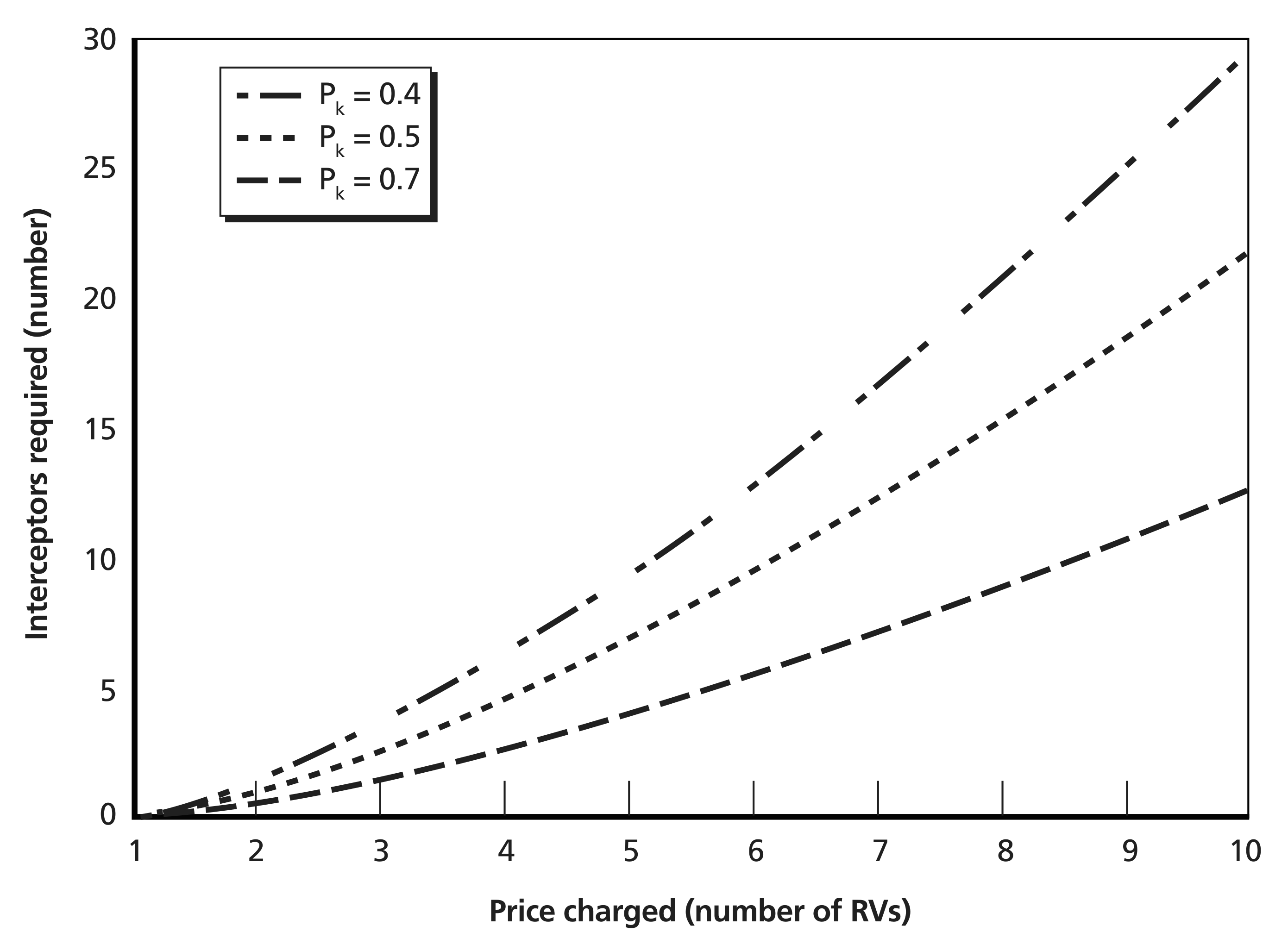
|
With this “analog
computer,” calculating the number of interceptors required
became a simple matter of reading values off of a graph.
Once you
understand the construct, the rest is easy:
1.
Postulate λ, the ratio of W
to
p.
The smaller the value chosen for λ, the larger the price you
must charge for a target of a given worth.
2. Decide how many DGZ areas you intend to defend.
3.
Calculate how many interceptors are required for each DGZ. This
number depends on the λ you have chosen, the worth of that
particular DGZ, the Pk
of
the interceptor, and the number of objects (RVs and decoys) in each
missile. In the example above, since each Soviet missile carried ten
objects (one RV and nine decoys) and the Nike-X radar could not
distinguish between RVs and decoys, the total number of interceptors
required to charge a price of four is 4.59 * 10 = 45.9.
Now
make a plot of the worth destroyed as a function of the number of
Soviet missiles in the attack. For this, I put the number of Soviet
missiles on the abscissa and “worth destroyed” for the
defended areas on the ordinate. This is a straight line starting at
the origin and at a slope of λ.
The line ends at the total worth contained in the “defended
areas.” If the Soviet attack includes the “undefended
areas,” tack on the worth destroyed per missile expended in the
undefended areas.
If
you have defended all “areas” whose worth is equal to or
greater than λ, the marginal return of worth for each Soviet
missile expended is exactly λ at the juncture of the lines of
defended and undefended areas.
An example of
such a plot is shown in Figure 6.2.
|
Figure
6.2 – Comparison of Worth Destroyed for Two Cases
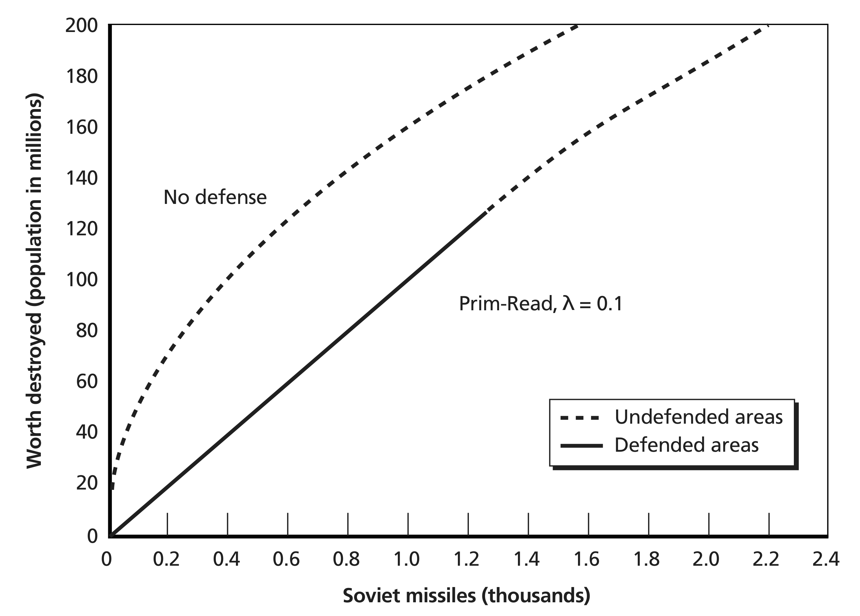
|
The figure
reflects calculations of worth destroyed as a function of the size of
a Soviet attack for two cases: (1) no defense and (2) a defense that
allocates interceptors according to the logic of Prim-Read. Both
cases in this somewhat notional example assume a target set
containing 1,600 DGZ areas and a total population of 200 million. The
distribution of the total population among the 1,600 DGZ areas is
assumed to obey a Pareto distribution with an exponent of one-half.
That is,
WCUM = 200 * (n / 1600)^0.5
or
WCUM = 5 * SQRT(n)
where
WCUM
is
the cumulative worth and n
is
the number of targets over which “worth” has been
accumulated. In the no-defense case, this relationship is also what
defines worth
destroyed
as
Soviet missiles are traded one-for-one with DGZ areas, starting with
the most lucrative areas to maximize the “expected return”
of each missile.
In
the case of the Prim-Read defense, λ
has
been set at 0.1. Thus, we want to defend DGZ areas up to the point
where the “expected return” of Soviet missiles is 0.1
million per missile. The next issue that arises is how many targets
we should defend. This question can be addressed target by target,
but I find it convenient to work with sets of targets instead. Since
cumulative worth obeys a Pareto distribution with an exponent of
one-half, we can define 40 sets (40 being the square root of 1,600)
with the following properties:
1.
The number of targets in the kth
set is equal to 2k
-
1. The first set contains the most valuable target; the second set
contains the next three most valuable targets; the third set contains
the next five most valuable targets; and so on.
2.
The number of targets through the kth
set is equal to k2.
There are four targets in the first two sets, nine targets in the
first three sets, 16 targets in the first four sets, and so on.
3. All sets are equal in value. Although each set
contains a different number of targets, the value of the first set
5
* SQRT(1) = 5
is the same as
the value of the 40th set
[5
* SQRT(40^2) ] - [5 * SQRT(39^2) ] = 5
and every set in
between. This is simply the total worth of the target set divided by
the number of sets, which is the square root of the total number of
targets. In this example, each set contains a worth of 5 million.
Since
λ
=
0.1 and since each set has a worth of 5 million, the defense should
charge a price of 50 for each set to be defended. If there are more
than 50 targets in a set, it does not need to be defended, since the
expected return per missile in that set would be less than 0.1. The
25th set contains 49 targets (2 ×
25
- 1 = 49). The 26th set contains 51 targets (2 ×
26
- 1 = 51). The expected return per missile expended in the 25th set
is slightly greater than 0.1, and it is slightly less than 0.1 in the
26th set. Thus, we defend 25 sets containing 625 targets with a
population of 125 million. The remaining 15 sets (975 targets with a
population of 75 million) are left undefended.
In
the absence of a defense, the Soviets could destroy half the total
worth of the target set by attacking the 400 most lucrative areas
with 400 missiles. In the presence of a Prim-Read defense with λ
=
0.1, the Soviets would need 1,000 missiles to inflict the same level
of damage. Moreover, only defended areas would be targeted, since
attacking these DGZs brings the highest “expected returns”
for Soviet RVs and the attack is not large enough to expect to
destroy the total worth in the defended areas (a population of 125
million). Undefended areas would be left alone unless the Soviet
attacks involved more than 1,250 missiles.
It
is worth noting that, while the defense significantly raises the
price of achieving a specified level of damage, it is not an
inexpensive proposition for the defender. For example, the third set
contains five targets with a population of 5 million. The population
of an average target within the set is 1 million. Since λ
=
0.1, the defender should charge a price of 10 for the average target,
which would require 21.8 interceptors for the average target. Thus,
roughly 109 interceptors are required to defend the set of five
targets if there are no decoys or if the radar can distinguish
between RVs and decoys. If we assume, as before, that each Soviet
missile in the attack carries one warhead and nine decoys and that
the Nike-X radar cannot discriminate between RVs and decoys, roughly
1,090 interceptors would be required to defend the five DGZ areas in
the set. Around 11,000 interceptors would be required to cover the
625 defended DGZ areas.
Dr. Brown was
quite impressed. He directed that the Army use this construct. They
accepted the construct, but it took the Army’s contractor a
while before he could get the computer to do his bidding.
Accordingly, I spent a good deal of time doing “what-ifs”
using a spreadsheet I had developed and a Friden calculator.
Doing “what-if”
calculations on a target-by-target basis would have been extremely
time consuming. After wrestling with the problem for a bit, I
realized that I could reduce my workload substantially if I used a
Pareto distribution with an exponent of one-half to represent the
distribution of worth among U.S. targets. I could then take advantage
of the properties of the distribution to define equal-value sets of
targets. I placed the most valuable target in the first set, the next
three most valuable targets in the second set, the next five most
valuable targets in the third set, and so on. The total number of
sets was equal to the square root of the total number of targets. For
each set I calculated the number of interceptors required to charge
the desired price for an average target and then multiplied by the
number of targets in the set to determine the total number of
interceptors required to defend the set. The set-based approach
dramatically reduced the number of “rows” required on a
spreadsheet. It was far easier and much faster to have to work only
with, for example, 40 sets instead of 1,600 individual targets. My
“turn time” was about two or three hours.
With a high-speed
computer to run the spreadsheet, the turn time could have been
reduced to minutes. Accordingly, Dr. Brown directed the Army to
instruct its contractor to do the “what-ifs” by running
my spreadsheet with a high-speed computer. Following several
unsuccessful attempts by the Army’s contractor, Dr. Brown
turned to the Institute for Defense Analyses (IDA) to do the
“what-ifs.” IDA’s project leader then made a
serious mistake. Instead of running the spreadsheet, he chose to
render a critique of the whole calculus. He let a contract to this
end to a professor of mathematics at New York University. This
professor’s finding: While Colonel Kent’s methodology may
be appealing on some counts, it has no firm foundation
mathematically.
The professor
offered a construct that had two features: (1) It would not work in
terms of deriving the relationship among size of attack, interceptors
deployed, and worth destroyed, and (2) it gave wrong answers for
items you could calculate. He had made a careless error in signs: He
had a plus when it should have been a minus.
Both Bob Prim and
Thornton Read were infuriated at this report. After all, it was their
construct that the professor had criticized. Dr. Prim went directly
to Dr. Brown. IDA was again directed to do the “what-ifs,”
but with no changes as to the spreadsheets.
The Prim-Read
theory still stands as an exceptional piece of work. Analysts over
the years have amended the calculus so as to account for noninteger
solutions. (The defense cannot fire 1.59 interceptors at an object.)
But the basic construct still stands. It was my luck to come across
it and use if to good effect.
And so it was
that my involvement in the calculus of the contribution of active
defense led to thinking about the contribution of other means of
limiting damage to the United States from attack by nuclear-armed
ICBMs: (1) counterforce operations, (2) active defense, and (3)
passive measures. This led to the defining study, “Limiting
Damage to the United States,” pp. 43-50.
Page 226 -230
The Trade-Offs Between Numbers,
Yield, and CEP in Hard-Target Kill
From time to time (in fact, too often according to my tastes), the
AFSC program office for ballistic missiles would present to the Air
Staff proposals to modify and modernize the Minuteman missile. During
my tenure in AFSA, the Ballistic Missile Office (BMO) often sought to
increase the HTK capability of the Minuteman force. HTK was defined
as the number of Soviet missile silos that could be attacked by the
Minuteman force with a damage expectancy of 0.9.
HTK can be increased in the following ways:
increasing the yield of the warhead, which entailed a newer
design and the use of more enriched uranium in each warhead
decreasing the CEP using a new and improved guidance system
simply increasing the number of missiles deployed
pursuing some combination of all three approaches.
I was generally skeptical of these proposals. In the first place,
the argument for seeking more HTK was not compelling: Even if the
United States were to launch a first strike, the relationship between
increased HTK and significantly reduced damage to the United States
was obscure. The second problem with the proposals had to do with the
“packaging” of increased yield, improved accuracy, and
greater numbers of warheads into a single proposal. BMO’s
presentations about the contribution of each component to the overall
measure of merit were always opaque.
To gain insight into these matters, I developed the following
construct:
The measure of merit is the number of Soviet silos attacked
at a stated DE of 0.9.
The probability that a Soviet silo will survive an attack by
one U.S. RV, Ps , is given by
Ps = 0.5^(LR^2 / C^2)
where LR is the lethal radius of the warhead, and C is
the CEP of the RV.
LR = λy^(1/3)
where λ is hardness of the silo.
The hardness of the Soviet silo, λ, was denoted as the
lethal radius of a single 1-megaton warhead. Thus, if a 1-megaton
warhead had a lethal radius of 1,000 feet, an 8-megaton warhead
would have an LR of 2,000 feet, since
³√(8)
= 2
Given these conditions, the Ps of a Soviet silo from an attack by
a single warhead was
Then, the Ps from n RVs against one silo would be
If we demand a DE of 0.9, it means that the exponent for 0.5 in
the equations must have the value of 3.32 (since 0.5^3.32 = 0.10).
Now we can gain some insight as to the relative contributions to
the total HTK of each of the measures proposed:
(400 / 250)^(2/3) =
1.37
If you decrease the CEP by a factor of 1.2, you will increase
the value of the exponent by a factor of 1.44, that is,
(1.2)^2
= 1.44.
You can gain the same increase in the value of the exponent
(namely, a factor of 1.44) by deploying 1.44 times as many
deliverable RVs.
The first two measures (increasing the yield and decreasing the
CEP) resulted in a combined increase of HTK by a factor of 1.97. In
their presentation to the Air Staff, the BMO staff packaged the two
measures together and stated that their proposal would “leverage
the force by almost double.” But they were silent about the
relative contribution of each measure. The total bill for their
proposed program was, even by BMO’s own estimates, quite large,
and I believed that their estimates were grossly understated.
General Ryan asked me to evaluate BMO’s proposal. In my
briefing to him I confirmed that increasing the yield of the
Minuteman warhead from 250 to 400 kt and reducing the CEP by a factor
of 1.2 would, indeed, double the HTK of the Minuteman force. But I
went on to point out that the majority of this increase in HTK
stemmed from improving the guidance system, while the great majority
of the cost of BMO’s proposal came from developing and
deploying a new RV. This was so because many launches of the missile
with the new warhead would be needed to test the RV’s ballistic
properties and because large amounts of enriched uranium would have
to be procured. According to my figures, the ratio of costs (of the
new RV versus the new guidance system) was six to one. Based on my
analysis, the Chief of Staff and the Secretary of the Air Force
approved a program to develop the new guidance system for the
Minuteman, but they did not approve a program for the new RV.
The above demonstrates that simple constructs can provide insight
and reliably inform decisions about whether or not to proceed to
implement some concept being proposed.
This episode was but one of a continuing battle between some
members of the Air Staff and the ballistic missile program office.
BMO continually sought funding to proceed with the development of a
new RV for Minuteman, and I prevailed on the issue throughout my
tenure in AFSA. However, subsequent to my departure from AFSA, a new
Chief of Staff did grant approval to proceed with a new RV. The
program was hardly a success—a large cost overrun occurred, and
the resulting RV failed to meet its expected performance
specification with respect to its yield.
The Trade-Off with “Soft” Area Targets
Now examine the trade-off between yield and numbers for the case
of attacking “soft” area targets. Such targets include
industrial infrastructure and unhardened military targets. In this
case, the trade-off between numbers and yield is not so obvious. If
the area occupied by the target is very large compared to the lethal
area of one weapon, then the trade-off is the same:
(n*y)^(2/3)
where n is the number of RVs and y is the yield of each.
But that is seldom the case; industrial facilities are generally
built not in large, circular clusters but rather more on a line
(e.g., along a river or railroad within a valley). If the facilities
lie in a line whose width is less than the diameter of the lethal
area of the weapon, then we can, by math, announce the trade-off:
(n*y)^(1/3)
The one-third term in the exponent results from the fact that some
of the weapon’s effects are expended outside of the target
area. We have now bounded the problem: The exponent of y is somewhere
between 0.33 and 0.67.
One might be tempted to take the arithmetic mean between these two
values—0.5—but there would be a hue and cry about
mathematical inelegance. So I devised a more complicated method for
arriving at the answer. Specifically, I devised a chart with “Soviet
value destroyed” on the ordinate and “number of weapons”
on the abscissa and, for a family of curves, yields of 100, 200, 500,
1,000, and 2,000 kt. It took some effort to construct the lines, but
finally we had the chart. Obviously, all lines (one line for each
yield) started at zero and were concave downward—reflecting the
fact that, as you went to more and more weapons on the abscissa, you
were attacking targets of less and less value and thus for
diminishing returns. Obviously, the 1-megaton lines rose more rapidly
than the lines for lesser yields.
Now the trick: Draw a horizontal line from some place midway up
the ordinate. This is a line of constant value destroyed. For
example, we note that, for the line of 200 kt, it took 800 weapons to
achieve this level of damage, and that, for the 1-megaton line, it
took only 360 weapons. Now find the value of z so that 0.200^z
× 800 is equal to 1^z
× 360. The answer is z
= 0.5. That is, when the exponent is 0.5, the square root
of 0.200 × 800 = 358—close
enough. Obviously, I took some other numbers and did not get the same
value for z for all pairs. But the average value for the exponent was
about 0.5—maybe a little less.
I now have stored in my mind that the exponent to use in
determining the trade between numbers of weapons (n) and the yield of
each (y) is Y^0.5 for
the case of soft area targets. As we saw earlier, this relationship
comes in handy in gaining insight into problems such as determining
the number of RVs on the front end of the Minuteman III missile (see
pp. 144—146).